CRYSOUND POCKET Acoustic Imaging Camera Now Available on Kickstarter.


Blogs
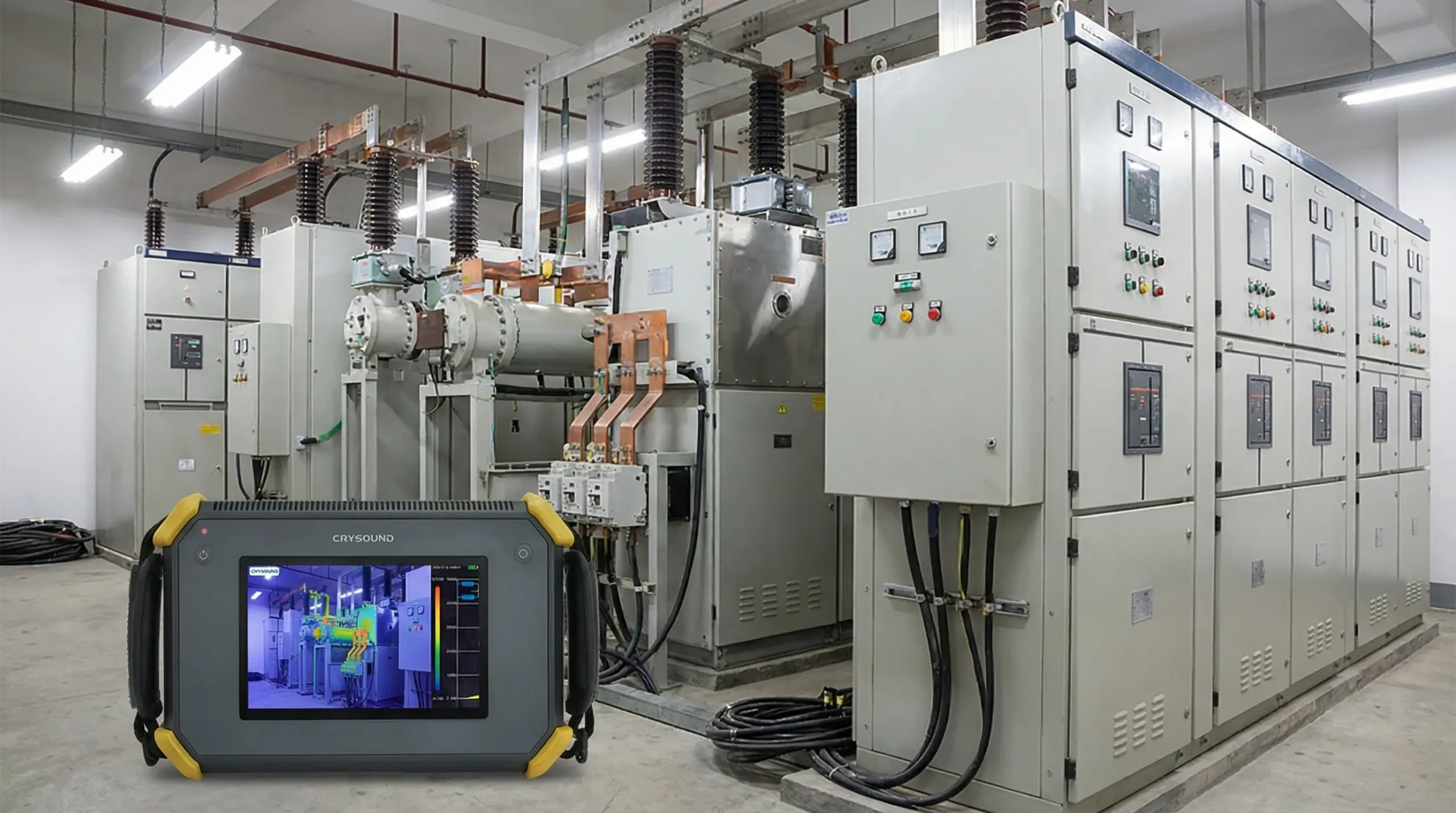
Partial discharge (PD) signals were detected in the medium-voltage switchgear of a plant, raising concerns about the safety and stability of the electrical system. To ensure safe inspection, the technical team isolated the affected area by cutting power. Corrective measures included applying high voltage from an external source to the equipment and using advanced detection tools to accurately identify the location and root cause of the discharge. During the investigation, two main methods were employed to detect and analyze PD signals: Ultrasound Transient Earth Voltage (TEV) Detection and Diagnosis Floating Partial Discharge (PD) signals were detected at the medium-voltage switchgear panels of a plant using EA UltraTEV Plus² with Ultrasound and Transient Earth Voltage (TEV) methods. However, the exact location of the PD could not be determined. Figure 1. TEV measurement showing a 30 dB floating pattern in MV switchgear, indicating likely internal partial discharge. Figure 2. Ultrasound measurement showing a 26 dBμV PD pattern in MV switchgear with clustered discharge activity. Pinpointing the Source with CRY2623 To further investigate, high voltage from an external source was applied to the circuit breaker within the open switchgear panel. The CRYSOUND CRY2623 device — capable of recording partial discharge signals in the form of images, sound, and diagrams — was then used to visually and accurately identify the precise source of the discharge signals. As a result, the plant's power outage time was significantly reduced. Figure 3. CRY2623 acoustic imaging locating floating PD at the upper pole field deflector of the circuit breaker. Root Cause Identified The source of PD signal was identified at the field deflectors of the upper pole of the circuit breaker. Upon inspection, it was discovered that the field deflector was loose and showed signs of no contact with the busbar, due to the rubber O-ring beneath the deflector being thinner than the design specification. Figure 4. Inspection showing the thin O-ring beneath the field deflector, identified as the root cause of floating PD. Verification After Repair A thicker rubber O-ring was installed as a replacement. After re-energizing the equipment, the partial discharge (PD) signal was rechecked to verify improvement. Figure 5. Repair showing replacement with a thicker O-ring beneath the field deflector to correct floating PD. Figure 6. Post-repair ultrasound and TEV results showing noise-level ultrasound and 5 dB TEV with no concern. The CRYSOUND CRY2623 acoustic imaging camera enables engineers to accurately localize partial discharge sources in real time - reducing diagnostic time, minimizing unplanned downtime, and keeping your electrical systems running safely. Whether you're dealing with switchgear, transformers, or cables, the CRY2623 delivers fast, reliable fault detection so you can act before small issues become costly failures. Interested in learning more? Fill in the Get in touch form below and our team will get back to you shortly. About the Author PSTS (Vietnam) – PSTS is a trusted partner providing industrial maintenance equipment (online and offline) and advanced CBM solutions to enhance customer asset safety and reliability throughout their life cycle. Website: https://psts.co
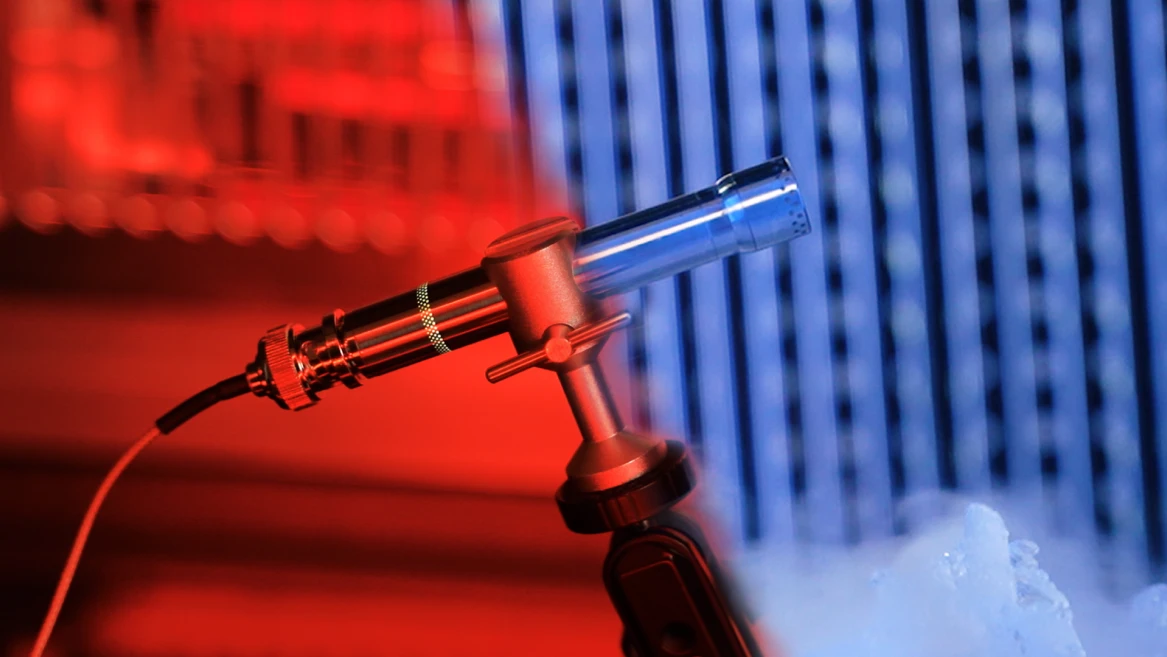
CRY3213 is a 1/2-inch prepolarized free-field microphone engineered for NVH testing in the real world — rain, dust, engine bay heat, Arctic cold. With IP67 protection and a -50°C to +125°C operating range, it delivers lab-grade accuracy without compromise, from powertrain noise to road and wind noise measurements. The Problem With Traditional Microphones Every NVH engineer knows the frustration: you need accurate acoustic data, but the test environment is anything but laboratory-perfect. Rain. Dust. Engine bay heat at 120°C. Scandinavian winter at -40°C. Vibration. Shock. Road spray. Traditional measurement microphones weren't built for this. They're precision instruments designed for controlled environments — fragile, temperature-sensitive, and one drop away from an expensive recalibration. So engineers compromise: they protect the microphone instead of optimizing the measurement, or they accept degraded data from sensors pushed beyond their limits. CRY3213 changes this equation entirely. Figure 1. CRY3213 operating in harsh road test conditions — water, mud, and debris are no obstacle A Game Changer for NVH Testing The CRY3213 is the NVH measurement microphone that delivers laboratory-grade accuracy in the harshest real-world conditions — without compromise, without babysitting, without excuses. This isn't an incremental improvement. It's a new category: the ruggedized precision NVH microphone. FeatureWhat It Means for Your Testing-50°C to +125°C operating rangeTest in Arctic cold or next to a turbo manifold — same accuracy, same reliabilityIP67 dust & water protectionContinue operating in rain, road spray, temporary water immersion, sand and dust — without extra protectionRuggedized, vibration-resistant designSurvives the shocks and vibrations of real-world vehicle testing without signal degradation50 mV/Pa sensitivityHigh output for excellent signal-to-noise ratio, even in quiet cabin measurements3.15 Hz – 20 kHz (±2 dB)Full audible bandwidth plus infrasound — captures everything from tire cavity resonance to HVAC hiss Figure 2. CRY3213 performing in extreme weather road testing Why CRY3213 Is Different Extreme Temperature Performance Most measurement microphones spec a conservative operating range. That's fine for a lab. It's useless for: Cold climate testing in Arjeplog, Sweden (-35°C) or Northern China (-40°C) Under-hood measurements where temperatures routinely exceed 100°C near exhaust manifolds and turbochargers Thermal cycling tests that swing from frozen to furnace in minutes CRY3213 operates at -50°C to +125°C with specified accuracy. No warm-up drift. No thermal shutdown. No recalibration needed between temperature extremes. When your competitors are swapping frozen microphones in the parking lot, your CRY3213 is still collecting data. IP67: Truly Weatherproof IP67 means:- 6 = Total dust ingress protection (dust-tight)- 7 = Protected against temporary immersion in water (up to 1 meter, 30 minutes) For NVH testing, this translates to:- Pass-by noise testing in rain — no test cancellations, no scrambling for covers- Road spray and puddle testing — mount microphones at wheel height without worry- Tropical humidity environments — no condensation-related signal drift- Outdoor long-term monitoring — deploy and forget CRY3213's IP67 is the highest protection class available in a precision NVH microphone. Figure 3. CRY3213 IP67 waterproof immersion testing Ruggedized and Vibration-Resistant Traditional condenser microphones are inherently precise and delicate. The CRY3213 has been systematically reinforced at the structural level for field durability, allowing it not only to measure near the vehicle, but also to be mounted directly on the vehicle for testing. Shock-resistant structural design helps withstand field handling and repeated installation/removal. Power-on LED indication enables quick confirmation of the microphone's operating status. Vibration-isolated design helps suppress mechanical interference transmitted through test benches and vehicle structures. The cable and connector system is designed for frequent connection, disconnection, and field deployment. No-Compromise Acoustic Performance Ruggedized doesn't mean reduced performance. CRY3213 delivers: Sensitivity: 50 mV/Pa (-26 dB re 1V/Pa) — matching premium lab microphones Frequency Response: 3.15 Hz to 20 kHz (±2 dB) — the full NVH bandwidth Dynamic range 17 to 136 dB — handles everything from quiet cabin to high-SPL engine bay measurements Low-frequency extension to 3.15 Hz — critical for tire cavity resonance (180–250 Hz), body boom (30–60 Hz), and powertrain low-order vibrations Prepolarized design — no external polarization voltage needed; plug-and-play with any IEPE/CCP input Application Scenarios Automotive NVH — Where CRY3213 Shines ApplicationChallengeCRY3213 AdvantagePowertrain NoiseEngine bay, 80–120°C, heavy vibrationTemperature range + vibration resistanceRoad Noise TestingOutdoor, all weather, road sprayIP67 + wide temperature rangeWind Noise TestingWind tunnel or outdoor, high airflowRuggedized + dust protectionPass-by Noise (ISO 362)Outdoor, rain or shine, year-roundIP67 enables all-weather testingCold Climate ValidationArctic conditions, -30°C to -50°C-50°C low-end operating rangeEV Motor Whine AnalysisNear e-drive, electromagnetic interferenceHigh sensitivity + vibration isolationSqueak & RattleInterior, door panels, dashboardFull bandwidth down to 3.15 HzProduction Line EOL TestFactory floor, dust, temperature swingsIP67 + rugged design for 24/7 industrial use Beyond the automotive industry, the CRY3213 is also well suited to aerospace, rail transportation, heavy industry, and the energy sector. Typical applications include engine ground run testing, interior and exterior train noise measurements, compressor and turbine noise monitoring, and wind turbine noise assessment under extreme weather conditions. Figure 4. CRY3213 installed in engine bay for powertrain noise testing Technical Specifications ParameterSpecificationType1/2" Free-field, PrepolarizedIEC StandardIEC 61094 WS2FSensitivity (±2 dB)50 mV/Pa, -26 dB re 1V/PaFrequency Response (±2 dB)3.15 Hz – 20 kHzDynamic Range (re. 20 µPa)17 dB(A) – 136 dBPower SupplyIEPE (2–20 mA)ConnectorBNCOperating Temperature-50°C to +125°CStorage Temperature-25°C to +70°COperating Humidity0–90% RH, non-condensingIP RatingIP67 (dust-tight, waterproof)Dimensions (with grid)Ø14.5 mm × 92 mmPolarization0 V (prepolarized)Weight36 g Frequently Asked Questions Q: Can I use CRY3213 with my existing NVH data acquisition system?A: Yes. CRY3213 is a prepolarized (0V) IEPE/CCP microphone, compatible with any standard constant-current input — including systems from SonoDAQ, CRY6151B, Siemens (SCADAS), HBK (LAN-XI), Dewesoft, National Instruments, HEAD acoustics, and others. Q: How does it handle rapid temperature changes during thermal cycling tests?A: CRY3213 is designed for continuous operation across its full -50°C to +125°C range, including rapid transitions. The thermal compensation ensures sensitivity stability without requiring recalibration between temperature extremes. Q: Is it suitable for permanent outdoor installation?A: Yes. With IP67 protection, CRY3213 is suitable for long-term outdoor deployment. Q: What's the advantage over ordinary microphones for NVH?A: Compared with conventional microphones, the CRY3213 NVH microphone not only delivers more accurate measurements, but is also better suited for real-world testing conditions. With IP67 protection, an operating temperature range of -50°C to +125°C, and excellent resistance to vibration and shock, it can operate reliably in rain, dust, high heat, and extreme cold, making it ideal for vehicle road tests, under-hood measurements, and long-term outdoor monitoring. Q: 10-year warranty — what does it cover?A: CRYSOUND's 10-year warranty covers manufacturing defects and sensitivity drift beyond specification. It's one of the longest warranties in the measurement microphone industry, reflecting our confidence in CRY3213's long-term reliability. Ready to Upgrade Your NVH Testing? Stop compromising between precision and durability. CRY3213 delivers both. Request a Quote → Download Datasheet (PDF) → Compare All CRYSOUND Microphones →
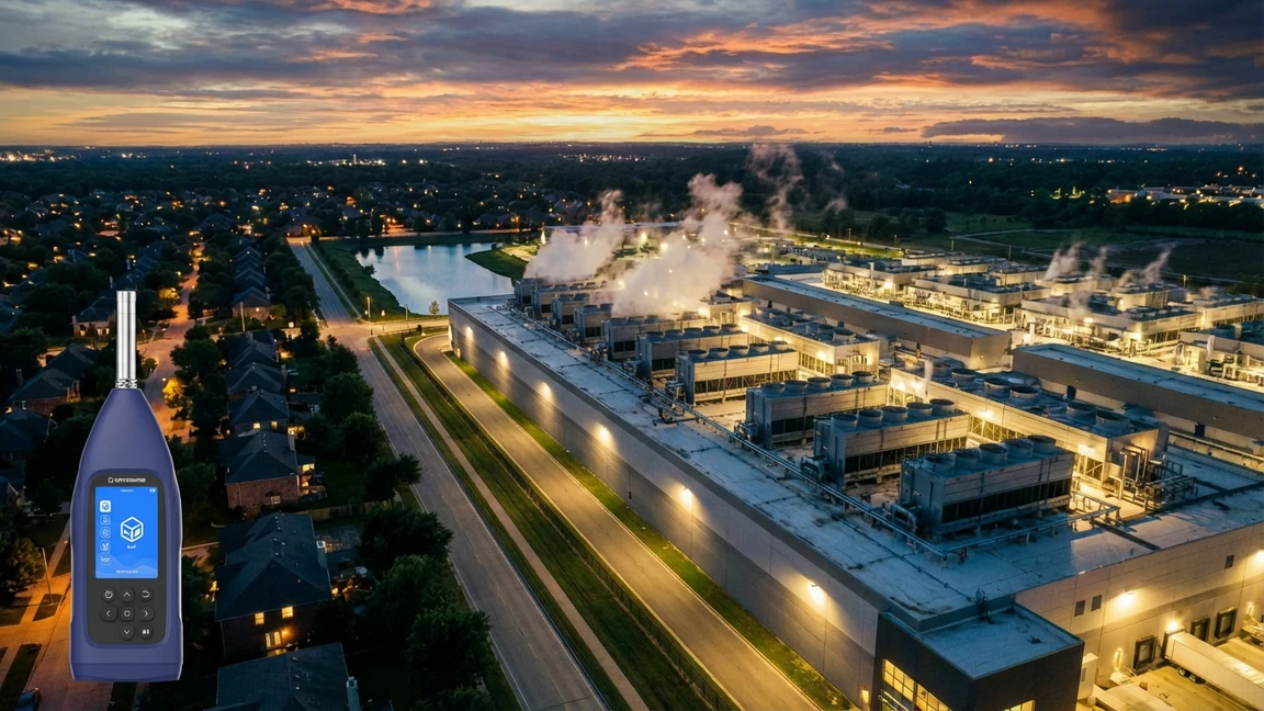
CRYSOUND's CRY2830 Series sound level meters support 24/7 data center noise monitoring, helping operators maintain noise compliance records and reduce the risk of fines. As AI workloads surge and hyperscale facilities continue to expand, data center noise complaints are rising rapidly. At the same time, environmental noise regulations are becoming more stringent. In Europe, more than 109 million people - about 20% of the population - are exposed to environmental noise above 55 dB(A). Driven by compliance requirements, the acoustic analysis services market is also growing quickly, with a projected CAGR of 6.4% through 2035. This is no longer just a matter of being a good neighbor. It is now a hard compliance requirement. Without continuous monitoring, operators are essentially flying blind. Figure 1. Site overview related to data center noise monitoring and property boundary compliance. Why Data Center Noise Is Becoming a Regulatory Priority Data center noise is not just annoying - it is a public health issue. The World Health Organization has noted that chronic noise exposure above 53 dB Lden is associated with significantly higher risks of hypertension, stroke, and heart attack. Regulations in multiple regions are tightening at a visible pace: LocationRegulationKey RequirementAurora, IL, USANew Data Center Ordinance (2026)24/7 automatic noise monitoring at the property line; daytime limit of 55 dB(A), nighttime limit of 45 dB(A)Prince William County, VA, USANoise Ordinance Update (2025)Noise limits for data centers; fines of $250-$500 per violationEuropean UnionEnvironmental Noise DirectiveNoise mapping, action plans, and a 55 dB(A) Lden threshold The trend is clear: what used to rely on self-discipline is quickly becoming a legal obligation. Figure 2. Environmental context relevant to data center noise compliance and surrounding sensitive areas. The Real Cost of Non-Compliance A fine of $250 to $500 per violation may not look serious for billion-dollar operators, but the actual cost goes far beyond the amount of the penalty itself: Project delays and permit rejection: Projects that cannot prove noise compliance at the planning stage may be rejected or delayed indefinitely. High retrofit costs: Emergency installation of acoustic enclosures after community complaints is extremely expensive, while early sound level assessment during design and operation can prevent that cost. Damage to reputation and community relations: Noise complaints erode community goodwill faster than almost any other issue. Operational restrictions: Some ordinances may force operators to reduce cooling capacity at night, directly affecting uptime and SLA commitments. Using the CRY2830 Series to Take Control Continuous noise monitoring is not only about compliance - it is about proactive control. For the demanding requirements of 24/7 outdoor monitoring in data centers, ordinary handheld instruments are not enough. The CRYSOUND CRY2830 Series sound level meters, when used with the dedicated outdoor protection kit, provide a practical high-accuracy solution for long-term compliance monitoring. Meets international standards for defensible reporting The foundation of compliance is reliable and legally defensible data. The CRY2833 sound level meter meets IEC 61672-1:2013 Class 1 requirements, helping ensure that reports submitted to regulators are credible, traceable, and technically sound. Outdoor protection for long-term boundary monitoring A sound level meter used at the property boundary must operate continuously in outdoor conditions. When paired with the NA41 outdoor protection kit, the system reaches IP65 protection, helping resist dust and water splashes. Its windscreen can still reduce wind noise by more than 30 dB at 10 m/s, which is especially important for capturing real equipment noise in harsh weather conditions. Figure 3. CRY2833 and CRY2834 with windscreen for outdoor data center noise monitoring. Captures low-frequency hum with octave analysis One of the most common complaints around data centers is the low-frequency hum generated by cooling equipment in the 63-250 Hz range. Standard A-weighted measurement can underestimate this problem. The CRY2830 Series supports both 1/1 octave and 1/3 octave analysis, making it easier to identify and evaluate these hidden low-frequency noise sources. Continuous logging and alarm-ready monitoring The system includes a built-in 32 GB microSD card for continuous data logging, with data automatically saved in standard CSV format. This makes it easier to build long-term compliance records and export measurement data for review. Flexible connectivity and system integration The CRY2830 Series also offers multiple interfaces, including Bluetooth, WiFi, RS232, and USB, making it easier to integrate sound level data into an existing BMS or cloud dashboard for remote access and long-term management. Figure 4. CRY2833 and CRY2834 interface options for data logging and system integration. Best Practices for Deployment Start with a baseline survey: Before installing permanent monitoring equipment, carry out a full noise survey to establish background noise levels and identify dominant noise sources. Use strategic placement with outdoor protection: Deploy the CRY2833 with the NA41 outdoor protection kit at property boundary points closest to sensitive receivers such as residential areas. Monitor low-frequency noise and use smart triggers: Enable 1/3 octave analysis to flag low-frequency issues and set threshold-based triggers for automatic recording when needed. Generate compliance-ready records: Export standard CSV measurement data regularly so that you have a defensible record available for any future noise complaint or regulatory review. Conclusion The data center industry is reaching a turning point. Regulations are tightening, and the cost of non-compliance already far exceeds the investment required for a professional sound monitoring system. 24/7 sound level monitoring is not a regulatory burden - it is an operational advantage. It gives operators better data, better decisions, stronger community relations, and written proof that they are doing the right thing. To learn more, explore the CRY2830 Series and contact CRYSOUND for a customized data center noise compliance solution.

By Bowen · Application Engineer at CRYSOUND Compressed air leaks rarely announce themselves as a major failure. More often, they sit in the background: a hiss at a fitting, a loss point on an overhead run, a manifold that never seems quite stable, a line that stays pressurized when it does not need to. Small individually. Expensive in aggregate. That is why leaks are easy to underestimate. They do not always stop production, but they do keep drawing power and eroding usable system capacity day after day. The U.S. Department of Energy and ENERGY STAR both note that leaks can account for roughly 20% to 30% of compressed air system output in a typical plant, and ENERGY STAR adds that poorly maintained systems may lose 20% to 50% of their compressed air to leaks. A compressed air leak cost calculator can help quantify that burden. Once losses reach that range, the issue is no longer housekeeping. It is an operating-cost problem and a maintenance-priority problem. Why air leaks cost more than they look Air leaks cost more than they look because they consume both electricity and capacity. The obvious loss is energy: compressors are producing air the plant never uses. The less obvious loss is system headroom. When enough air escapes through avoidable leaks, the plant may start seeing pressure instability, slower recovery after peak demand, or equipment that feels short of air even though compressor capacity on paper should be adequate. That is why leaks often surface as symptoms before they are treated as root causes. Teams may notice unstable downstream pressure, poor actuator response, longer recovery time, or compressors that seem to be working harder than expected. The first reaction is often to adjust pressure setpoints, add capacity, or tune controls. Sometimes the simpler truth is that too much air is leaving the system before it ever reaches productive use. Compressed air leak cost: the yearly operating cost associated with compressed air that your system generates, but your plant never uses because it escapes through avoidable leaks. ENERGY STAR draws a useful contrast here. In a plant with an active leak program, losses may be kept below 10%. In a poorly maintained system, the leak share can be far higher. That gap turns leaks from background noise into a measurable operating expense. Where compressed air leaks usually hide in real plants In most plants, compressed air does not disappear through one spectacular failure. It leaks away through ordinary connection points that are easy to ignore because each one looks minor on its own. Typical leak locations include: quick-connect fittings and couplings hoses and hose-end connections threaded joints FRL assemblies and valve manifolds drains, traps, and condensate components aging seals in cylinders or actuators idle machines that stay pressurized when they do not need to be overhead distribution lines that are physically hard to inspect Some of these are simple bench-level fixes. Others are difficult mainly because of access and visibility. Overhead piping, dense manifolds, crowded mechanical spaces, and background noise all make it harder to localize the exact point of loss quickly. That is one reason leak programs stall even when everybody agrees the system probably has leaks. Why teams know leaks exist but still struggle to fix them Most plants do not lack awareness. They lack a repeatable path from suspicion to action. There are several reasons for that: the leak burden is spread across many assets rather than one dramatic failure background plant noise makes traditional listening unreliable overhead or crowded geometry slows inspection maintenance teams are asked to prioritize problems that look more urgent leadership may not see a clear financial case for dedicating time to a leak campaign Leak programs often fail at the handoff between engineering intuition and operational prioritization. The maintenance team may know leaks are present. The plant may even hear them. But if nobody can frame the cost clearly enough to justify time, and nobody can localize the leaks efficiently enough to repair them, the issue stays on the backlog. A calculator helps with the first half of that problem. It does not solve the leak. It tells the plant whether the leak problem is large enough to deserve immediate attention. Use our free calculator to estimate the business impact This article includes a lightweight compressed air leak cost calculator for that decision point. It is meant to answer one practical planning question: If our leak burden is in a realistic range, what could it be costing us per year? It supports two simple input paths: Estimate from compressor data if you know installed power, electricity cost, and runtime assumptions Use annual electricity cost if you already know the approximate yearly electricity spend for your compressed air system Compressed Air ROI How much are air leaks costing your plant? Estimate the annual cost of compressed air leaks in less than a minute. Switch between a compressor-data estimate and a direct electricity-cost shortcut. Typical planning assumption 20% Estimated leak loss rate Use the leak-loss slider to model your plant. The calculator updates live so you can stress-test different assumptions before planning repairs. Estimate from compressor data Use annual electricity cost Input assumptions Use the path that best matches what you already know about your compressed air system. Currency Affects result formatting only USD ($) EUR (€) GBP (£) CNY (¥) Total installed compressor power HP kW Electricity cost per kWh Repair budget (optional) Operating days per week Operating hours per day Annual non-production days Currency Match your annual electricity cost input USD ($) EUR (€) GBP (£) CNY (¥) Annual compressed air electricity cost Repair budget (optional) Estimated annual cost of air leaks $0 Adjust the inputs to see how compressed air leaks can turn into recurring annual spend. Annual air-system electricity cost $0 Average monthly leak cost $0 Average daily leak cost $0 Estimated payback period — Planning estimate only. This calculator helps you frame the possible business impact of compressed air leaks. It does not replace a plant energy audit or a quantified leak survey. Want to find the leaks behind this cost? Acoustic imaging helps maintenance teams see compressed air leaks faster on manifolds, fittings, and overhead lines. See acoustic leak detection solutions Assumption note: leak-loss percentage is user-defined so teams can model conservative or aggressive scenarios. The key input is the estimated leak-loss rate. That percentage is intentionally scenario-based because plants start from very different conditions. A well-managed system may justify a lower case. A site with legacy piping, recurring fitting changes, idle assets left pressurized, and no regular survey routine may justify a higher one. Use the output for planning, not for forensic accounting. Its job is to convert a suspected problem into an estimated annual exposure that can support budgeting, prioritization, and a decision on whether a leak survey should move up the queue. Why finding the leak matters more than estimating it A cost estimate is only useful if it changes field behavior. Once a plant sees that leaks may be costing thousands or tens of thousands of dollars per year, the real operational question becomes: Can we find the leaks fast enough to repair them without turning the program into a slow manual hunt? This is where many leak initiatives bog down. Estimating cost is relatively easy compared with localizing leaks across real plant geometry. A few leaks near eye level may be obvious. A larger system with overhead runs, crowded manifolds, complex drops, and tight mechanical spaces is harder. Knowing that leaks exist is not the same as being able to repair them efficiently. Execution quality depends on localization speed. If finding leaks is painfully slow, even a strong energy-saving case can lose momentum. If localization is fast and repeatable, the plant can move much more confidently from estimate to inspection to repair. How acoustic imaging helps maintenance teams localize leaks faster DOE and ENERGY STAR guidance often point maintenance teams toward ultrasonic leak detection because escaping compressed air produces high-frequency sound that is easier to detect ultrasonically than by ear in a noisy environment. That is the right starting point. In the field, though, the hard part is often not detecting that sound. It is locating the exact source quickly on a live plant floor. Acoustic imaging helps by turning that signal into a visual map. Instead of relying only on point-by-point audio cues, the inspector can see where sound energy is concentrated on top of the live scene. On dense manifolds, fittings, hose assemblies, overhead lines, and hard-to-reach drops, that visual layer can make leak localization faster and easier to document. That is especially useful when: the suspected leak zone contains many possible connection points the leak is above eye level or across a congested mechanical area the team needs to document findings for a maintenance backlog multiple leaks must be ranked and repaired efficiently If you want a fundamentals refresher on the method itself, CRYSOUND already explains the basics in What Is an Acoustic Camera? and How Acoustic Imaging Works. Some acoustic imaging workflows also support leak-severity assessment, which matters when a plant is trying to prioritize repairs instead of treating every leak as equal. For plants doing regular compressed-air inspections, CRYSOUND's handheld lineup fits that workflow directly: the CRY8124 Advanced Acoustic Imaging Camera provides a higher-resolution handheld option with 200 microphones and a 2-100 kHz frequency range, while the CRY2623 128-Mic Industrial Acoustic Imaging Camera offers 128 microphones, a 2-48 kHz frequency range, and support for gas/vacuum leak detection and leak rating in a rugged industrial format. Plants do not buy inspection tools because leak math is interesting. They buy them because once the cost is visible, they need a practical way to find and fix the leaks behind the number. A practical workflow: estimate → inspect → repair → verify Once the plant accepts that leaks are carrying real cost, the next steps do not need to be complicated. Estimate the exposure. Use the calculator to test low, mid, and high leak-loss scenarios and decide whether the annual burden justifies focused action. Inspect the likely problem zones. Start with compressors, dryers, headers, manifolds, drops, hoses, valve packs, and idle equipment that stays pressurized. Repair the most valuable leaks first. Rank issues by probable severity, accessibility, safety, and operational impact rather than trying to fix everything at once. Verify and repeat. Re-inspect repaired areas, document recurring patterns, and turn leak detection into a maintenance routine instead of a one-off campaign. This workflow is deliberately practical. A plant does not need perfect certainty to start. It needs enough confidence that the waste is real, enough visibility to localize leaks efficiently, and enough follow-through to keep repairs from becoming a one-time campaign. FAQ How accurate is this compressed air leak cost calculator? It is a planning estimator, not an audit-grade model. Its job is to frame annual exposure quickly by using realistic operating assumptions and a user-defined leak-loss percentage. What leak-loss percentage should I start with? If you do not know your current leak level, 20% is a practical starting case. DOE and ENERGY STAR both identify that range as common enough to deserve attention, and you can compare it against lower and higher scenarios. Why not just estimate the savings and skip leak detection? Because the estimate does not tell you where the leaks are. Plants still need an inspection method that turns a cost problem into a repair list. When does acoustic imaging make the biggest difference? It is most useful when the leak is hard to localize quickly by ear or with manual point-by-point search, especially on overhead lines, dense manifolds, crowded mechanical spaces, and multiple-connection assemblies. Estimate the cost, locate the leaks, and turn the result into repairs. If your annual loss is already large enough to justify action, talk with CRYSOUND about acoustic leak detection solutions. Sources U.S. Department of Energy, Improve Compressed Air System Performance: A Sourcebook for Industry — https://www.energy.gov/eere/amo/improve-compressed-air-system-performance-sourcebook-industry ENERGY STAR, Compressed Air System Leaks — https://www.energystar.gov/industrial_plants/earn_recognition/small_manufacturing/guide/compressed_air_system_leaks U.S. Department of Energy, AIRMaster+ — https://www.energy.gov/eere/amo/articles/airmaster

As the core component of measurement chains, the long-term stability of measuring microphones directly impacts the comparability and traceability of measurement data. The 10-year limited warranty (hereinafter referred to as the 10-year warranty) is not merely a service commitment, but a comprehensive capability demonstrated through manufacturing consistency control, reliability verification systems, and traceable evidence chains. This article will outline the engineering implementation approach to explain the rationale behind CRYSOUND's 10-year warranty, and evaluate the impact of this warranty strategy on user lifecycle costs (including maintenance, logistics, downtime, and management costs) based on the Total Cost of Ownership (TCO) framework. Economic Value of 10-year Warranty: Budgeting Life Cycle Risk Cost For both laboratories and production lines, the "cost" of microphones constitutes only a fraction of total expenses. The bulk of costs stems from project downtime, retesting and rework, temporary replacements, cross-regional repairs, and administrative complexities. When the warranty period covers a larger portion of the equipment’s service life, users can plan risks and resources more clearly within lifecycle budgets. This is the true value of a Ten-Year Warranty. Engineering Foundation of 10-year Warranty: Reliability Design, Manufacturing and Verification System Manufacturing Process Capability and Consistency Control: Raw Material Validation and 102 Critical Processes Long-term stability primarily stems from consistency. CRYSOUND begins with raw material validation, preemptively identifying and eliminating risks such as corrosion resistance and insulation stability during the incoming material stage. Subsequently, each measuring microphone must undergo 102 stringent processes, with real-time monitoring during precision machining to ensure consistency in critical dimensions and fit. Selection of Critical Materials and Assembly Process Control: Physical Basis of Long-term Stability Key components are assembled by experienced technical experts, utilizing materials with high insulation and low temperature sensitivity to enhance environmental stability. As the core acoustic structure, the third-generation titanium diaphragm technology emphasizes performance objectives such as wide frequency response, high sensitivity, corrosion resistance, and magnetic insensitivity, employing structural and material design to mitigate long-term drift risks. Typical Failure Mechanism and Verification Coverage Matrix The long-term stability of microphones is typically compromised not by a single factor, but by cumulative effects of humidity, temperature, mechanical shocks, and contamination, leading to performance drift or noise degradation. Below is a comparison table illustrating how CRYSOUND maps these typical risks to manufacturing control points and factory verification: Typical risk/failure modeEngineering control pointCorresponding Verification / ScreeningMoisture causes noise to rise sensitivity fluctuationClean Assembly,Insulation Design and Process ControlHigh humidity prolonged test, insulation-related verification (sensitivity pre/post difference / base noise variation / insulation stability)Temperature change-induced driftMaterials and structural stability, assembly consistencyLong-term temperature cycling (sensitivity/frequency response changes, noise trends, structural and connection stability)Structural deflection caused by drop/vibrationStructural strength and assembly processDrop test, bidirectional vibration test (function output stability, key index difference before and after, structural integrity)Pollution/Particulate Matter Causes Noise DegradationUltrasonic cleaning, cleanroom commissioningComprehensive factory noise/performance testing (including noise floor, sensitivity, frequency response consistency, etc.)Corrosion/salt spray leads to reduced appearance and connection reliabilityCorrosion-resistant Material Screening, Surface Treatment and Connector Protection DesignSalt spray exposure/retention + Appearance and connection reliability verification Clean Manufacturing and Pollution Control: Noise and Long-term Stability Fine particles, oil contaminants, and impurities can amplify into noise elevation or performance fluctuations during prolonged use. To mitigate this, each measuring microphone undergoes ultrasonic cleaning and precision calibration in a cleanroom environment, thereby reducing the risk of contamination and foreign object introduction, ensuring low-noise and moisture-resistant performance at the source. Factory Reliability Verification Scheme: Environmental/Mechanical/Electrical Stress Verification A decade-long warranty hinges on systematic coverage of typical service environments and operational conditions. CRYSOUND's factory reliability verification adopts a fundamental approach of "representative environmental and mechanical stress coverage + critical risk coverage," categorizing verification items into three types: environmental stress (humidity, temperature cycling, salt spray), mechanical stress (drop/impact/vibration), and electrical reliability (insulation and leakage risks). This system screens and validates material, assembly, and connection weaknesses through stress coverage of humidity, temperature cycling, salt spray, and drop/vibration conditions before delivery, thereby reducing on-site failure risks. The high-humidity long-term validation examines how humidity affects microphone performance. Under controlled high-humidity conditions, the device undergoes continuous exposure to simulate prolonged moisture exposure, covering risks like insulation degradation, noise performance changes, and stability fluctuations. This is followed by retesting and electrical status verification to confirm the product's stability and consistency under thermal-humidity stress. High and Low Temperature Cycling Validation addresses structural and assembly robustness risks under temperature variation conditions. By conducting prolonged cycles between extreme temperature extremes, it accelerates exposure to potential issues including material thermal expansion differences, stress release, and joint stability. The engineering objective of this validation is to assess performance drift risks and connection/assembly stability under long-term temperature disturbances, thereby reducing the probability of post-delivery anomalies triggered by thermal stress. Salt spray testing addresses material and joint reliability risks in coastal, high-salt, or corrosive environments. By exposing components to controlled salt spray conditions, it evaluates the corrosion resistance of metal parts, joints, and protective designs. The process also includes visual inspection of joints and functional/electrical verification, effectively mitigating corrosion-induced reliability degradation and long-term stability risks. Note: Salt spray validation is used to evaluate the robustness of protection and connection under typical exposure conditions. For long-term operation in harsh environments such as strong corrosion or high salt spray conditions that exceed the product's usage specifications, additional protection measures must be implemented, with the warranty terms as the ultimate reference. Mechanical stress verification (Drop/vibration/Shock) addresses mechanical disturbance risks during transportation, installation, disassembly, and field operation. It involves simulating repeated 1-meter drop handling and accidental impacts through specified cycles, replicating transportation vibrations and prolonged mechanical disturbances via continuous vibration tests, and assessing transient stresses under higher intensity through impact validation. The core objective of mechanical verification is to screen structural integrity, assembly stability, and connection reliability, thereby reducing post-delivery risks of intermittent anomalies and performance variations caused by micro-loosening, connector stress, or assembly misalignment. As a baseline control for electrical reliability, insulation verification addresses risks of leakage, breakdown, or instability caused by moisture, pollution, and material aging. It verifies the insulation performance of critical electrical paths and, when necessary, conducts post-stress environmental reviews to ensure the product maintains stable electrical safety and signal reliability throughout its lifecycle. All aforementioned validation items are implemented in accordance with the company's internal factory inspection specifications, accompanied by procedures for anomaly isolation, re-inspection, and disposal. Products identified with anomalies during the validation process will not proceed to the delivery phase. CRYSOUND 10-year warranty key points Main pointsExplanationScope of applicationApplicable to 3000 series: microphones, preamplifiers, kits, dummy mouthpieces, dummy earpieces, and complete sets (traceable via nameplate/serial number).Warranty Duration DifferencesThe main equipment typically has a lifespan of ten years; accessories/consumables (such as wind shields, cables, connectors, seals, etc.) have a lifespan of six months and should be separately included in the maintenance budget.Start methodPriority is determined by the outbound/delivery date; if no voucher is available, by the end user's purchase date; if still unavailable, by the last date traceable by the factory date or serial number.Warranty contentConfirm material or process defects: Free repair (necessary parts + labor) or replacement with the same model/performance equivalent to the original (possibly certified refurbishment/remanufacturing).Typical non-protectionMisuse/abuse, drop and compression, liquid immersion, corrosive gases/salt spray, overvoltage/reverse connection/ESD/surge, unauthorized disassembly/repair, etc.Calibration apertureCalibration drift within the specified range is a common phenomenon in metrology and does not constitute a manufacturing defect; calibration/recalibration is typically a paid service (unless the drift is confirmed to be caused by a manufacturing defect).Logistics and Cross-borderDefault rule: Users within the warranty scope are responsible for round-trip shipping costs. Cross-border transactions may incur tariffs, customs clearance fees, or taxes, which are typically borne by the user unless otherwise agreed in the contract. Visit https://www.crysound.com/warranty for more information How A Ten-Year Warranty Affects TCO: Cost Structure and Budget Strategy TCO scope and boundary conditions The TCO (Total Cost of Ownership) discussed herein refers to the "total cost" of equipment throughout its lifecycle, encompassing not only the purchase price but also measurement and maintenance, logistics turnover, downtime, and management costs. It is crucial to clarify that warranty coverage addresses "failure risks caused by material/process defects," while calibration/recalibration focuses on "measurement traceability and drift management." Unless testing confirms drift stems from manufacturing defects, calibration/recalibration and measurement certificate updates are typically not covered by free warranty. Users should budget for these as annual predictable costs. Meanwhile, logistics and cross-border costs related to repairs/services should be factored into the TCO calculation upfront. By default, users are responsible for round-trip shipping within the warranty period. Cross-border transactions may incur tariffs, customs clearance fees, or taxes, which are typically borne by the user unless otherwise stipulated in the contract. TCO cost decomposition model and accounting subject A simple model can help you understand the lifecycle cost of a microphone. TCO = Procurement cost + Calibration/recalibration cost + Logistics/cross-border cost + Consumables and accessories replacement + Unplanned downtime/re-testing/rework + Management cost (ledger/compliance/traceability) The Impact of 10-year Warranty on Risk-related Costs: Emergency Expenditure Reduction and Management Cost Optimization Cost reduction for unplanned maintenance/replacement: Material/process defects triggering repairs or replacements are covered by the warranty mechanism, reducing the likelihood of unexpected expenses and emergency procurement. Reduced downtime and retest/rework costs: With enhanced equipment stability and manageable risks during the warranty period, projects experience fewer instances of temporary failures, abnormal fluctuations, or the need for downtime, retesting, or rework. Reduced diagnostic and communication costs: Serial number traceability, historical data, and certificate records can lower localization costs, minimize unnecessary back-and-forth and redundant testing, and enhance processing efficiency. Projected operating costs: annual budget proposal Calibration/Recalibration (annual budgeting recommended): Minor drift in measuring instruments is normal. It is recommended to calibrate at least once every 12 months or as required by the system; verification or recalibration should be performed after high humidity, high temperature, strong vibration, or frequent disassembly and assembly. Supplies/Consumables (replenishment budget recommended): Windproof covers, cables, seals, etc. should be procured according to consumables regulations and replacement cycles to avoid downtime and temporary procurement costs caused by 'small components'. Logistics/International (budget should be allocated separately by scenario): By default, round-trip shipping costs, international customs duties, and clearance fees should be included in advance, especially for multi-location projects and cross-border scenarios. 10-year TCO estimation template Use the table below to quickly build your TCO estimate for procurement or asset inventory: Cost elementInput/AssumptionNotes (How to be affected by the 10-year warranty)Equipment procurementQuantity, Unit Price (RMB per unit)Procurement price is not the whole picture, but it determines the asset baseline Annual calibration/recalibrationFrequency (times/year), per-visit cost (yuan)Typically paid; recommended at least once every 12 monthsAttachments/SuppliesReplacement cycle and unit pricePlan according to the 6-month/consumable ruleLogistics/InternationalRound-trip freight, customs duties and clearanceThe default user assumes responsibility; cross-border scenarios require a separate listingDowntime costCost per outage, annual occurrencesReliability Improvement and Quality Assurance to Reduce the Probability of Unplanned OutagesRetest and reworkSingle rework cost, annual occurrencePerformance and Stability Reduction,Rework and Controversy Cost Accompanying Management of 10-year Warranty: Usage, Calibration and Asset Ledger Asset ledger and traceability information management: serial number—certificate—data association Enter the serial number and model (photograph for archiving), and bind the calibration certificate with factory data. Record critical operating conditions: temperature and humidity, presence of strong vibrations, and frequency of disassembly and assembly. When an exception occurs, prioritize reproducing the standard steps and retaining records (screenshots, waveforms, or comparison data). Usage and Handling Guidelines: Reducing Non-Guarantee Risks Avoid drops, compression, liquid immersion, and corrosive environments; power supply and connections shall be performed in accordance with the instructions. Unauthorized disassembly and repair are strictly prohibited. Ensure the nameplate/serial number is clearly identifiable. Use the original packaging or equivalent protective measures during repair/reinspection, and install protective covers/dust caps on precision interfaces. Repair Information List: Shorten the Location and Processing Cycle Model and serial number photos; purchase/delivery certificates. Fault description (scenario, frequency, environmental conditions, power supply and connection method). Reproducible test records (frequency response, sensitivity, noise, distortion, or system screenshots/waveforms). Conclusion: Ten-year warranty engineering logic and user value The ten-year warranty is built upon a verifiable, traceable, and operational engineering closed loop: reducing consistency risks through manufacturing process capability control, covering typical failure scenarios via environmental and mechanical stress validation, and supporting warranty determination and service efficiency with serial numbers and data records. For users, its value lies not only in fault handling itself but also in reducing the uncertainty of unplanned downtime and emergency replacements, making the lifecycle cost of measurement systems more predictable and easier to incorporate into annual budget management.
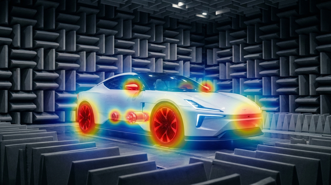
Traditional NVH tools still matter, but they don't cover every EV scenario—acoustic cameras fill the gap with real-time noise visualization and wide-band diagnostics. The Quiet EV Paradox: Why Electric Cars Are Actually "Noisier" It sounds like a paradox — electric vehicles have no roaring engine, yet engineers are finding it harder than ever to achieve a truly quiet cabin. The truth is, when the low-frequency masking effect of the internal combustion engine disappears, every previously hidden noise becomes fully exposed: the high-frequency whine of the electric motor, the electromagnetic hum of the inverter, gear meshing vibrations, wind noise, road noise, even the squeak and rattle of interior trim — nothing can hide anymore. This isn't just a comfort issue. It's fundamentally redefining the automotive industry's approach to NVH (Noise, Vibration, and Harshness) testing. The global automotive NVH testing market is projected to grow from USD 3.51 billion in 2026 to USD 5.75 billion by 2034, at a CAGR of 6.4%. The core driver behind this growth? The electrification revolution. What New Noise Challenges Do EVs Bring? A Fundamental Shift in Frequency Range Traditional ICE vehicle NVH work focuses on the 20–2,000 Hz low-frequency range — engine firing, exhaust systems, crankshaft vibrations. Electric vehicles are fundamentally different: Noise SourceTypical Frequency RangeCharacteristicsElectric motor electromagnetic noise500–5,000 HzSharp tonal noise, varies linearly with speedInverter switching noise4,000–10,000+ HzHigh-frequency hum, related to PWM frequencyGear meshing noise800–3,000 HzParticularly prominent in single-speed reducersBattery charger noise8,000–20,000 HzNear-ultrasonic range, at the edge of human perceptionWind / Road noise200–4,000 HzHighly exposed without engine masking ICE vs EV: The fundamental shift in noise frequency characteristics Key insight: EV noise problems shift from low frequencies to mid-high frequencies (and even ultrasonic ranges). The 100Hz-5kHz range is where most critical NVH issues reside—precisely where human hearing is most sensitive. Traditional NVH testing methods and frequency ranges may no longer be sufficient. New Noise Sources, New Localization Challenges In the ICE era, the assumption that "the engine is the dominant noise source" made things relatively straightforward. In EVs, noise sources become more distributed and complex: Electric drive system: The motor + inverter + reducer form a highly coupled noise system Thermal management: Battery cooling pumps and fans become dominant noise sources at low speeds Regenerative braking: Changes in inverter operating modes during energy recovery produce transient noise Structural transmission paths: Lightweight body structures (aluminum alloy, carbon fiber) have fundamentally different sound insulation characteristics compared to traditional steel This means engineers face a core challenge: How do you quickly and accurately locate the root cause among multiple distributed, dynamically changing noise sources? Sound Quality Design: From "Reducing Noise" to "Crafting Sound" NVH engineering in the EV era is no longer just about "minimizing noise." Consumers expect a carefully designed sound experience: Acceleration should feel "high-tech" without being harsh The cabin should be quiet, but not so silent that it makes the driver uneasy Different driving modes (Sport / Comfort / Eco) should deliver differentiated acoustic feedback This demand for "Sound Design" is expanding NVH testing from pure engineering validation into subjective sound quality evaluation and brand-level acoustic identity. Why Acoustic Cameras Are Becoming Essential for EV NVH Facing these new challenges, traditional NVH testing tools — single-point microphones, accelerometers — remain important but are no longer sufficient for every scenario. Acoustic cameras are filling this gap. Core Advantages of Acoustic Cameras 1. Real-Time Noise Source Visualization Traditional methods require densely placing microphone arrays on the target object — time-consuming and labor-intensive. Acoustic cameras use beamforming technology to generate a noise source heatmap in a single capture, instantly showing "where the noise is and how loud it is." Typical scenario: An EV prototype running on a test bench, the acoustic camera aimed at the electric drive system, instantly revealing that an 800 Hz resonance originates primarily from the right side of the motor — the entire localization process takes less than 5 minutes. Engineer conducting noise source localization test Automotive NVH detection and optimization 2. Wide Frequency Coverage EV noise spans from hundreds of hertz (gear meshing) to tens of thousands of hertz (inverter switching noise) — an enormous frequency range. Critical consideration for NVH: Most EV noise issues occur in the 100Hz-5kHz range—gear meshing, motor electromagnetic noise, wind leaks, HVAC systems. Traditional acoustic imaging cameras (limited to frequencies above 5 kHz) cannot capture these noise sources. Take the CRYSOUND SonoCam Pi (CRY8500 Series) as the ideal example: its 208 MEMS microphone array provides: Beamforming frequency range: 400 Hz - 20 kHz (covers the entire NVH audible spectrum) Near-field acoustic holography range: 40 Hz - 20 kHz (captures low-frequency road noise and structural vibration) Array size: >30 cm (optimized for low-frequency spatial resolution) This makes SonoCam Pi uniquely suited for full-spectrum EV NVH testing—from low-frequency road noise to high-frequency motor whine, all in a single handheld device. 3. Non-Contact Measurement EV electric drive systems are highly integrated and spatially compact. The non-contact measurement approach of acoustic cameras means: No disassembly of any components required No interference with the operating state of the system under test Rapid quality inspection directly on the production line 4. Portability Modern handheld acoustic cameras like the SonoCam Pi can be taken directly to proving grounds, production lines, or customer sites, no complex setup required. Typical Application Scenarios in EV NVH ScenarioApplicationE-drive system NVHLocating order-based noise contributions from motors, inverters, and reducersPass-by noise testingAnalyzing noise source distribution as vehicles pass byInterior squeak & rattle trackingLocating noise from dashboards, doors, seats, and trimEnd-of-line production QCRapid online detection of abnormal noise, replacing subjective human judgmentWind tunnel / Semi-anechoic chamberHigh-precision noise source localization and sound power analysis Real-World Case Study: OEM Dynamic Road Testing Client: A leading Chinese OEMLocation: An OEM test center, internal test trackObjective: Identify in-cabin noise sources during dynamic driving conditions CRY8500 Series SonoCam Pi acoustic cameras Test Setup Device:SonoCam Pi acoustic camera Measurement positions:Rear seat and front passenger seat Target areas:Left and right B-pillars (rear cabin area) Test mode:Beamforming app Frequency range:3,550 Hz - 7,550 Hz Dynamic range:5 dB Key Results SonoCam Pi successfully localized noise sources in real-time during vehicle motion, providing actionable data for OEM's NVH engineering team. The test demonstrated: Real-time localization during dynamic conditions: Unlike fixed laboratory setups, SonoCam Pi captured noise distribution while the vehicle was in motion on the test track Precise frequency-band analysis: By focusing on the 3,550-7,550 Hz range (critical for perceived cabin noise), engineers pinpointed specific contributors rather than measuring overall SPL Rapid testing workflow: Complete B-pillar area scan in minutes, not hours Noise Source Localization Results Key Insight: Traditional microphone arrays would require the vehicle to be stationary in a semi-anechoic chamber. SonoCam Pi enabled on-track diagnostics, dramatically reducing testing time and enabling rapid iteration during vehicle development. Future Trends — What's Next for EV NVH Testing? AI-Driven Noise Classification Machine learning is being integrated into NVH testing workflows: automatically identifying noise types, determining whether anomalies exist, and predicting potential quality issues. The high-dimensional data captured by acoustic cameras is naturally suited for AI analysis. Digital Twins and Simulation-Test Integration Simulation (CAE) predicts noise performance → Acoustic camera validates through physical measurement → Data feeds back to optimize the simulation model. This closed-loop approach is becoming the standard workflow for major OEMs. New Challenges in the Solid-State Battery Era Solid-state batteries have different mechanical properties compared to liquid lithium-ion batteries. Their vibration transmission characteristics and thermal management approaches will introduce new NVH challenges. Stricter Regulations Pass-by noise testing is the fastest-growing NVH sub-segment (CAGR 7.11%), with UNECE pushing for stricter standardized testing requirements, including indoor pass-by testing protocols. Conclusion: The Value of Acoustic Testing, Redefined for the EV Era Electrification hasn't made cars quieter — it has made noise challenges more complex, more nuanced, and more valuable to solve. For automotive OEMs, Tier 1 suppliers, and testing service providers, investing in the right NVH testing equipment is no longer a "nice-to-have" — it's foundational infrastructure for competitiveness. Acoustic cameras—especially those capable of capturing the critical 100Hz-5kHz NVH frequency range—are evolving from "useful auxiliary tools" to "indispensable standard equipment." The CRYSOUND SonoCam Pi stands out as the only handheld acoustic camera that combines: Low-frequency capability (400 Hz beamforming, 40 Hz holography) High spatial resolution (208 microphones, >30 cm array) Near-field + far-field measurements in a single system Portability (handheld, <3 kg, production-ready) Learn more: CRYSOUND SonoCam Pi (CRY8500 Series) → Contact us for NVH testing solutions →
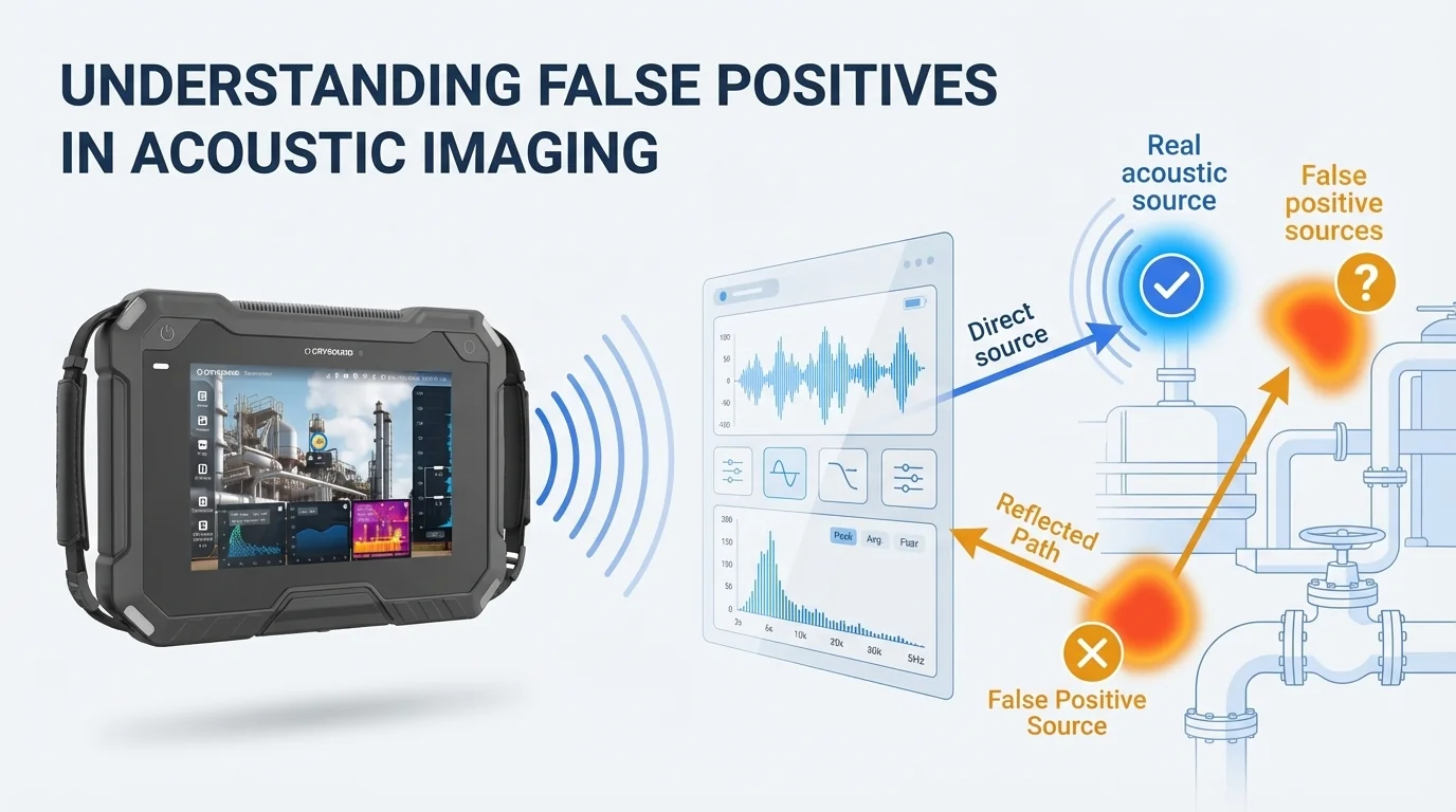
You're scanning overhead pipework in a compressor room when your acoustic camera shows a bright hotspot on a steel support beam. You walk over, listen carefully, and check the surface. Nothing. No hiss, no vibration, no leak. The image looks convincing, but the source is not actually on that beam. This is one of the most common acoustic imaging false positives engineers see in the field. Acoustic camera reflections, beamforming artifacts, and background noise can all create ghost images or false hotspots that look like real leaks, discharges, or mechanical faults. That does not mean the camera is malfunctioning. It means the operator needs to separate true sources from indirect paths and side responses. Based on field observations in reflective industrial environments, teams often find that 15–30% of initial acoustic indications should be treated as leads for verification rather than confirmed source locations. In this guide, we'll explain why an acoustic camera shows false hotspots, how to tell acoustic camera reflections from real leaks, and how to reduce beamforming artifacts in noisy factories without slowing down your inspection workflow. What Are False Positives in Acoustic Imaging? False positive (acoustic imaging): An apparent sound source indication on an acoustic camera display that does not correspond to an actual physical source at that location. Caused by physical phenomena including sound wave reflections, beamforming algorithm sidelobes, or environmental noise interference — not by equipment defect. Three related terms often get used interchangeably, but they describe different phenomena: False positive: Any indicated source that isn't real at the shown location Artifact: A systematic error pattern produced by the beamforming algorithm itself (e.g., sidelobes) Ghost image: A reflected or mirrored source — real sound arriving from an indirect path Understanding these distinctions matters because each type has different causes, different on-screen characteristics, and different solutions. Why Acoustic Cameras Show False Hotspots If your acoustic camera shows a hotspot on a wall, support beam, enclosure, or ceiling panel, the most common cause is a reflection rather than a leak at that exact surface. In other words, the hotspot may still be useful, but it is pointing to an indirect path instead of the true source location. If the display shows a halo, ring, or repeating spots around one strong source, that pattern is more likely a beamforming artifact than a second leak. And if the hotspot is broad, unstable, or spread across a noisy production area, environmental noise is usually a better explanation than a discrete defect. For teams using acoustic cameras in compressed air leak detection, it helps to pair this article with our acoustic camera guide and how acoustic imaging works explainer. If you need to quantify the cost of missed leaks before the next survey, use our air leak cost calculator. Common False Positives in Acoustic Cameras Reflections (Ghost Images) Sound waves bounce off hard, smooth surfaces — metal walls, concrete floors, glass panels, polished pipes — just like light reflects off a mirror. When your acoustic camera picks up both the direct sound and the reflected sound, the reflected path appears as a second source at a location where nothing is actually producing noise. Typical scenario: You're imaging a compressed air manifold mounted near a stainless steel wall. The display shows two hotspots — one on the manifold (real) and one on the wall behind it (ghost). The ghost image appears at roughly the same intensity and frequency as the real source. On-screen signature: Ghost images tend to appear at geometrically symmetrical positions relative to the reflecting surface. They share the same frequency spectrum as the real source and often appear at similar or slightly reduced intensity. Sidelobe Artifacts This is the most technically nuanced type. Beamforming algorithms work by mathematically "focusing" the microphone array on each point in the field of view. But just as a flashlight can't produce a perfectly sharp beam edge, beamforming produces a main lobe (the focused area) surrounded by sidelobes — weaker response regions that can register false sources. Typical scenario: You're imaging a single loud leak, but the display shows the main hotspot surrounded by a ring or pattern of secondary spots. These sidelobe artifacts are always clustered around the true source and become more pronounced when the source is loud relative to surrounding noise. On-screen signature: Sidelobes appear as a repeating pattern around the main source — often a ring, halo, or radial spoke pattern. Their intensity is always lower than the main lobe, and they maintain a fixed geometric relationship to the primary source regardless of scanning angle. Key factor: The number of microphone channels directly affects sidelobe levels. A 64-channel array produces more prominent sidelobes than a 128-channel array, which in turn produces more than a 200-channel array. Higher channel counts provide narrower main lobes and lower sidelobe floors. Advanced algorithms like CRYSOUND's HyperVision processing further suppress sidelobes beyond what standard delay-and-sum beamforming achieves. Environmental Noise Interference Not every unwanted indication is a reflection or algorithm artifact. Sometimes, your acoustic camera is accurately detecting a real sound — just not the one you're looking for. Background noise from HVAC systems, nearby machinery, overhead cranes, or even wind can register as apparent sources that get confused with your target. Typical scenario: During a compressed air leak survey in a manufacturing hall, you see multiple hotspots across a wide area. Some are genuine leaks. Others are background machinery noise that happens to fall within your selected frequency band. On-screen signature: Environmental noise sources typically have broader, more diffuse patterns than leaks (which appear as tight, focused hotspots). They also show different frequency characteristics — machinery noise tends to be narrower-band and harmonic, while leak noise is broadband and turbulent. Quick Comparison Type Cause On-Screen Signature Elimination Difficulty Reflections Sound bouncing off hard surfaces Symmetrical ghost image, same frequency as real source Moderate — multi-angle scan + frequency check Sidelobe artifacts Beamforming algorithm side response Ring/halo pattern around main source, lower intensity Low with advanced algorithms (HyperVision) Environmental noise Background machinery in frequency band Diffuse pattern, tonal/harmonic frequency profile Low — frequency filtering + Focus Function How to Identify False Positives: A 4-Step Process When you see an indication you're unsure about, run through these steps before logging it as a confirmed source: Angle change test. Move 2-3 meters to the side and re-scan the same area. Real sources stay in the same physical position on the image. Reflections shift or disappear as you change the angle of incidence. Sidelobes rotate with the main source. Frequency signature check. Switch to spectrum view (if your camera supports it) and examine the frequency profile. Compressed air leaks produce broadband, turbulent noise typically above 20 kHz. Machinery noise has distinct tonal peaks. If the "source" shares an identical spectrum with a known real source nearby, it's likely a reflection. Distance validation. If your camera allows distance-to-source measurement, check whether the indicated distance matches the physical geometry. A reflection off a wall 3 meters behind you will show a source distance that doesn't match the wall's position from your scanning location. Ultrasonic listening. Most acoustic cameras offer a downshift playback feature that converts the directionally-captured ultrasonic signal into audible sound through headphones. Point the camera at the suspect indication and listen. A real compressed air leak produces a distinctive broadband hiss. Sidelobe artifacts and reflections carry no independent acoustic signature — they sound identical to the main source. Environmental noise sounds tonal and harmonic. This lets you verify from your scanning position without walking to the indicated location. Techniques to Minimize False Positives 1. Select the Right Frequency Band Most acoustic cameras allow you to filter by frequency range. Narrowing the band to your target application reduces interference dramatically. For compressed air leaks, focus on 20–50 kHz. For partial discharge, 20–100 kHz. Excluding lower frequencies cuts out most machinery noise. 2. Use Advanced Beamforming Algorithms Not all beamforming is equal. Standard delay-and-sum (DAS) algorithms are computationally simple but produce higher sidelobe levels. Advanced algorithms apply spatial filtering to suppress sidelobes at the processing level. CRYSOUND's HyperVision algorithm, available on the CRY8124 and CRY8120 series, provides up to 10x processing power over standard beamforming, reducing sidelobe artifacts significantly without sacrificing real-time performance. 3. Adopt a Multi-Angle Scanning Protocol Make it standard practice to scan critical areas from at least two different positions. Compare the results. Sources that appear consistently in the same physical location are real. Sources that shift, disappear, or change intensity are false positives. This takes an extra 30 seconds per area and dramatically reduces misdiagnosis. Turning Artifacts into Allies: Using False Positives to Locate Sources Here's where experienced operators separate from beginners. False positives aren't just noise to eliminate — they carry information about the acoustic environment that you can exploit. Reflection Mapping If you see a ghost image on a metal wall, you've just learned something valuable: there's a real sound source at the geometrically mirrored position. The reflection tells you the sound wave's travel path. In complex piping environments where direct line-of-sight to a leak is blocked, reflected images on nearby surfaces can reveal the general direction and approximate distance of sources you can't see directly. Pro technique: When scanning in confined spaces with multiple reflective surfaces, intentionally note where ghost images appear. The pattern of reflections triangulates the true source location, even when the source is behind equipment or above a ceiling panel. Sidelobe Pattern Reading Sidelobes always radiate symmetrically from the main lobe. When you see a sidelobe pattern, the center of that pattern is your real source — guaranteed. In environments where obstructions partially block your view, the visible sidelobes can confirm the direction of a source that's partially hidden. If the sidelobe "ring" is only visible on one side, the true source is on the opposite side, behind whatever's blocking your view. Spatial Focusing (ROI Isolation) In noisy industrial environments, you can't shut down surrounding equipment just to get a cleaner acoustic image. Instead, use your camera's Focus Function: draw a region of interest (ROI) directly on the screen around the area you want to investigate. The camera restricts its beamforming analysis to that region only, effectively suppressing sound sources outside the selected area. This is particularly powerful when combined with frequency band filtering. Narrow the frequency range to your target application (e.g., 20–50 kHz for leak detection), then draw an ROI around the suspect zone. The double filter — spatial plus spectral — dramatically reduces environmental noise interference without requiring any change to the plant's operating conditions. What previously looked like a cluttered display with overlapping hotspots becomes a clean, focused view of the area that matters. Quick Reference Checklist Eliminating false positives: Set correct frequency band for target application Scan from at least two angles Check frequency spectrum of ambiguous sources Use ultrasonic listening to verify auditory signature before logging Leveraging false positives: Note reflection positions to triangulate hidden sources Read sidelobe patterns to confirm source direction Use Focus Function (ROI) to isolate target area from surrounding noise Need help diagnosing false positives? Talk to our application engineers → Frequently Asked Questions How common are false positives in acoustic imaging? Every acoustic camera produces some false positives. They are an inherent characteristic of beamforming physics, array geometry, and reflective environments rather than a product defect. With the right scanning workflow, most operators can tell a real source from a false hotspot within seconds. Why does my acoustic camera show a hotspot on the wall? The most common reason is reflection. The wall is acting like an acoustic mirror, so the camera detects indirect sound energy and maps it to the mirrored position. If the hotspot shifts or disappears when you change your scanning angle, you are likely looking at a reflection instead of a real source on that wall. What is the difference between a reflection and a beamforming artifact? A reflection is real sound reaching the array by an indirect path after bouncing off a surface. A beamforming artifact is a pattern generated by the imaging algorithm itself, often appearing as a halo or repeating side response around a strong source. Reflections usually move with geometry and angle; beamforming artifacts stay locked to the true source pattern. Can reflections be completely eliminated? No. As long as there are hard, smooth surfaces in the environment, sound will reflect. However, you can reduce their impact by scanning from multiple angles, matching spectra, and using region-of-interest controls to isolate the target area. Does a higher microphone channel count reduce artifacts? Yes. More channels generally provide a narrower main lobe and a lower sidelobe floor, which means fewer misleading side responses around strong sources. This is one reason acoustic camera specifications matter when you compare systems. How do I handle false positives in noisy factory environments? Use three filters together: narrow the frequency band to the target application, restrict the imaging area with an ROI or focus function, and confirm suspicious hotspots from a second angle. In most plants, that combination separates real leak-like sources from machinery noise fast enough for practical inspections. Can acoustic reflections actually help locate the real source? Yes. Reflections reveal the sound path, which means a ghost image can still tell you where to keep searching. In cluttered piping or enclosed machinery spaces, reflection patterns often help experienced operators triangulate the hidden source more quickly.
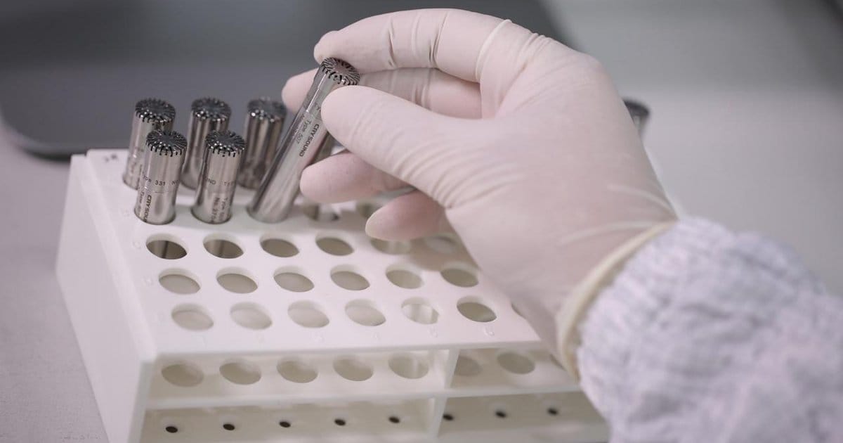
A measurement microphone is not just any microphone — it is a precision acoustic sensor designed for traceable, repeatable sound pressure measurement. This guide covers how they work, the different types available, key specifications to compare, and how to select the right one for your application. What Is a Measurement Microphone? A measurement microphone is a high-precision acoustic transducer engineered to convert sound pressure into an electrical signal with known accuracy. Unlike studio or consumer microphones that are designed to make audio "sound good," a measurement microphone is designed to be truthful — its output must faithfully represent the actual sound pressure at the measurement point. The defining characteristics of a measurement microphone include: Known, stable sensitivity (expressed in mV/Pa) that can be traced to national or international standards Flat, well-characterized frequency response under defined sound-field conditions Wide dynamic range with low distortion from noise floor to maximum SPL Traceable calibration using pistonphones or acoustic calibrators Environmental stability — minimal drift due to temperature, humidity, and atmospheric pressure changes In practical terms, a measurement microphone is the front-end sensor of a metrology-grade measurement chain. Every specification — from the data acquisition system to the analysis software — depends on the microphone providing an accurate representation of the acoustic environment. For a deeper comparison between measurement and regular microphones, see our article: Differences Between Measurement Microphones and Regular Microphones. How Measurement Microphones Work The Condenser Principle How a condenser measurement microphone converts sound pressure into an electrical signal Nearly all measurement microphones are condenser (capacitor) microphones. The core transduction mechanism is simple but elegant: A thin metallic diaphragm is stretched in front of a rigid backplate, separated by a small air gap The diaphragm and backplate form a capacitor When sound pressure deflects the diaphragm, the gap changes, altering the capacitance With a constant charge on the capacitor, the capacitance change produces a proportional voltage change This voltage change is the microphone's output signal. A preamplifier, typically located immediately behind the capsule, converts the high-impedance signal from the capacitor into a low-impedance signal that can travel through cables to the data acquisition system. Polarization: External vs. Prepolarized Externally polarized (left) vs. prepolarized electret (right) microphone types The condenser principle requires a polarization voltage to maintain a charge on the capacitor. There are two approaches: Externally polarized microphones receive their polarization voltage (typically 200V) from an external power supply through the preamplifier. These microphones are considered the gold standard for the highest-accuracy laboratory measurements because:- The polarization voltage is stable and well-defined- No aging effects from the polarization source- Best long-term stability Prepolarized (electret) microphones use a permanently charged PTFE (Teflon) layer on the backplate to maintain polarization. Advantages include:- No external polarization supply needed — simplifies the signal chain- More resistant to humidity (no risk of charge leakage at high humidity)- Better suited for field measurements and harsh environments- Modern prepolarized microphones achieve accuracy comparable to externally polarized models FeatureExternally PolarizedPrepolarizedPolarization sourceExternal 200V supplyBuilt-in electret layerBest forLab/reference measurementsField and industrial useHumidity toleranceSensitive above ~90% RHExcellent, even in high humidityLong-term stabilityExcellentVery good (modern designs)Signal chainRequires compatible power supplyWorks with standard IEPE/ICP preamplifiers The Preamplifier The preamplifier is a critical but often overlooked component. It serves two functions: Impedance conversion: Transforms the microphone's extremely high output impedance (~GΩ) into a low impedance suitable for cable transmission Signal conditioning: Provides the power for IEPE/ICP operation or the polarization voltage for externally polarized capsules A matched microphone-preamplifier set ensures optimal performance. This is why measurement microphones are often sold as complete sets with a matched preamplifier — the combined system is calibrated and characterized as a unit. Types of Measurement Microphones Measurement microphones are classified along two primary axes: sound-field type and physical size. By Sound-Field Type The choice of microphone type depends on the acoustic environment where measurements will be taken. Free-Field Microphones A free-field microphone is designed to measure sound arriving from a single direction in an environment free of reflections (such as an anechoic chamber or outdoors). The microphone's frequency response is compensated for the acoustic diffraction effects caused by its own physical presence in the sound field. When to use: Outdoor measurements, anechoic chamber testing, source identification, environmental noise monitoring, any scenario where sound arrives predominantly from one direction. Orientation: Point the microphone directly at the sound source (0° incidence). Pressure-Field Microphones A pressure-field microphone measures the actual sound pressure at a surface or in a sealed cavity. It has the flattest possible response when the sound field is uniform across the diaphragm — which occurs in small cavities, couplers, or at surfaces where the microphone is flush-mounted. When to use: Coupler measurements (headphone and earphone testing), hearing aid testing, measurements in small cavities, flush-mounted surface measurements, acoustic impedance measurements. Orientation: The microphone diaphragm is placed at or within the measurement surface. Random-Incidence Microphones A random-incidence (diffuse-field) microphone is optimized for environments where sound arrives from all directions simultaneously — such as reverberant rooms. Its frequency response is a weighted average of responses at all angles of incidence. When to use: Reverberation chamber measurements, environmental noise in reflective spaces, any situation where sound arrives from multiple directions. Microphone TypeSound FieldTypical ApplicationOrientationFree-fieldSound from one directionOutdoor noise, anechoic testing, source IDPoint at sourcePressure-fieldUniform pressure (cavity)Coupler testing, headphones, hearing aidsFlush with surfaceRandom-incidenceSound from all directionsReverberant rooms, diffuse environmentsAny orientation Three microphone types for different acoustic environments: free-field, pressure-field, and random-incidence By Physical Size Measurement microphone capsules come in three standard sizes, each with distinct trade-offs: 1-Inch Microphones The largest standard size. High sensitivity and low noise floor make them ideal for measuring very quiet environments. Sensitivity: ~50 mV/Pa (highest) Frequency range: Up to ~8–16 kHz Best for: Low-frequency and low-level measurements, environmental noise monitoring, building acoustics Limitation: Large size limits upper frequency range due to diffraction effects 1/2-Inch Microphones The most widely used size. Offers a good balance between sensitivity, frequency range, and physical size. Sensitivity: ~12.5–50 mV/Pa Frequency range: Up to 20–40 kHz Best for: General-purpose acoustic measurements, NVH testing, product R&D, sound level meters Why it's popular: Versatile enough for most applications; fits standard sound level meter bodies 1/4-Inch Microphones The smallest standard size. Low sensitivity but the widest frequency range. Sensitivity: ~1.6–16 mV/Pa Frequency range: Up to 40–100 kHz Best for: High-frequency measurements, ultrasonic applications, small coupler measurements, acoustic array elements Trade-off: Higher noise floor requires louder sound sources for accurate measurement Size comparison: 1-inch (CRY3101), 1/2-inch (CRY3203), and 1/4-inch (CRY3401) measurement microphone capsules SizeSensitivity (typical)Frequency RangeDynamic RangeBest For1 inch50 mV/Pa4 Hz – 16 kHz15–146 dBALow-frequency, quiet environments1/2 inch12.5–50 mV/Pa3 Hz – 40 kHz16–164 dBAGeneral-purpose, NVH, SLM1/4 inch1.6–16 mV/Pa4 Hz – 100 kHz32–174 dBAHigh-frequency, ultrasonic, arrays Key Specifications Explained When comparing measurement microphones, these specifications matter most: Sensitivity Sensitivity defines how much electrical output the microphone produces for a given sound pressure. Expressed in mV/Pa (millivolts per Pascal) or dB re 1V/Pa. Higher sensitivity = better signal-to-noise ratio at low sound levels Lower sensitivity = higher maximum SPL before distortion There is always a trade-off between sensitivity and maximum SPL Frequency Response The frequency range over which the microphone provides accurate measurements, typically specified within ±2 dB or ±1 dB. The useful range depends on:- Microphone size (smaller = wider range)- Sound-field type (free-field compensation extends the useful range)- Mounting configuration Dynamic Range The span between the lowest measurable level (noise floor) and the highest level before a specified distortion threshold (typically 3% THD). A wider dynamic range means the microphone can handle a greater variety of measurement scenarios. Self-Noise (Equivalent Noise Level) The inherent electrical noise of the microphone, expressed as an equivalent sound pressure level in dBA. Lower is better — critical for measuring quiet environments. 1-inch microphones: ~15–18 dBA (quietest) 1/2-inch microphones: ~16–28 dBA 1/4-inch microphones: ~32–46 dBA Stability and Temperature Coefficient Long-term sensitivity drift and sensitivity change with temperature. Important for:- Permanent monitoring installations (fixed outdoor microphones)- Measurements in extreme environments (engine test cells, climatic chambers)- Ensuring measurement results are comparable over months or years IEC Standards Compliance Measurement microphones are classified according to IEC 61094 series:- IEC 61094-1: Primary calibration by reciprocity method- IEC 61094-4: Specifications for working standard microphones (laboratory use)- IEC 61094-5: Working standard microphones for in-situ (field) use Sound level meters incorporating measurement microphones must comply with:- IEC 61672-1: Class 1 (precision) or Class 2 (general purpose) How to Choose the Right Measurement Microphone How to select the right measurement microphone for your application Step 1: Identify Your Sound Field Your Measurement ScenarioRecommended TypeOutdoor environmental noiseFree-fieldAnechoic chamber testingFree-fieldHeadphone/earphone couplerPressure-fieldHearing aid testingPressure-fieldReverberant roomRandom-incidenceSurface-mounted on a machinePressure-fieldGeneral factory noiseFree-field or random-incidence Step 2: Determine Required Frequency Range ApplicationMinimum Frequency RangeBuilding acoustics20 Hz – 8 kHzEnvironmental noise20 Hz – 12.5 kHzGeneral acoustic testing20 Hz – 20 kHzNVH (automotive)20 Hz – 20 kHzElectroacoustic product testing20 Hz – 40 kHzUltrasonic measurements20 Hz – 100 kHz Step 3: Match the Dynamic Range to Your Environment Quiet environments (recording studios, anechoic chambers): Choose high-sensitivity microphones (50 mV/Pa, 1/2" or 1") with low self-noise Industrial environments (factory floors, engine test cells): Choose lower-sensitivity microphones (4–12.5 mV/Pa, 1/4" or 1/2") with high maximum SPL Wide-range applications: Choose microphones with the widest dynamic range available Step 4: Consider Environmental Conditions High humidity or outdoor use: Prepolarized microphones are recommended Extreme temperatures: Check the microphone's operating temperature range and temperature coefficient Dusty or wet environments: Look for IP-rated solutions (e.g., IP67 for NVH field testing) Hazardous areas: Check for ATEX/IECEx certification if required Step 5: Evaluate the Complete System A measurement microphone does not work alone. Consider:- Preamplifier compatibility: Matched sets ensure specified performance- Data acquisition system: Input impedance, voltage range, and sampling rate must match- Calibration infrastructure: Do you have access to a pistonphone or acoustic calibrator?- Software ecosystem: Can your analysis software import calibration data and apply corrections? Applications Electroacoustic Product Testing Testing loudspeakers, headphones, earphones, and hearing aids requires microphones that can accurately capture the device's frequency response, distortion, and directivity. Pressure-field microphones are used in couplers (IEC 60318 ear simulators), while free-field microphones are used in anechoic chambers. Automotive and Aerospace NVH NVH (Noise, Vibration, and Harshness) engineers use measurement microphones to characterize cabin noise, identify noise sources, evaluate sound packages, and perform transfer path analysis. Requirements include wide frequency range, high dynamic range, and robustness for field use. Environmental and Community Noise Monitoring Long-term outdoor noise monitoring stations require microphones with excellent stability over months or years, low temperature sensitivity, and tolerance to humidity, rain, and wind. Windscreens and weather protection accessories are essential. Production Line Quality Control In manufacturing, measurement microphones integrated into automated test systems verify that every loudspeaker, headphone, or microphone meets specifications before shipping. Speed, repeatability, and consistency are critical — the microphone must produce identical results across thousands of units per day. Building and Architectural Acoustics Measuring reverberation time, sound insulation, and HVAC noise requires accurate low-frequency performance and the ability to work in diffuse sound fields. Random-incidence microphones are often preferred. Acoustic Research and Standards Laboratories Primary and secondary calibration laboratories, standards organizations, and university research groups require the highest-accuracy microphones — typically externally polarized, laboratory-grade capsules calibrated by reciprocity methods. Sound Source Localization and Beamforming Microphone arrays used in acoustic cameras and beamforming systems require large numbers of measurement microphones with tightly matched sensitivity and phase response. 1/4-inch microphones are preferred for arrays due to their small size and wide frequency range. For more on acoustic imaging technology, see our guide on acoustic cameras. Noise Regulation Compliance Regulatory compliance measurements — workplace noise (ISO 9612), environmental noise (ISO 1996), product noise emission (ISO 3744/3745) — require Class 1 or Class 2 measurement microphones as specified in IEC 61672. Documentation of calibration traceability is mandatory for compliance reporting. CRYSOUND Measurement Microphone Solutions CRYSOUND's CRY3000 series measurement microphones cover the full range of sizes, field types, and applications — from laboratory reference measurements to rugged field testing. Complete Size Coverage: 1/4", 1/2", and 1" ModelSizeField TypeSensitivityFrequency RangeApplicationCRY3101-S011"Free-field50 mV/Pa4 Hz – 16 kHzLow-frequency, quiet environmentsCRY3203-S011/2"Free-field50 mV/Pa3.15 Hz – 20 kHzGeneral acoustic testingCRY3261-S021/2"Free-field450 mV/Pa10 Hz – 16 kHzUltra-high sensitivityCRY3201-S011/2"Free-field12.5 mV/Pa3.15 Hz – 40 kHzExtended high-frequencyCRY3401-S011/4"Free-field15.8 mV/Pa4 Hz – 40 kHzHigh-frequency testingCRY3403-S011/4"Free-field4 mV/Pa4 Hz – 90 kHzUltrasonic measurementsCRY3202-S011/2"Pressure12.5 mV/Pa3.15 Hz – 20 kHzCoupler and cavity testingCRY34021/4"Pressure1.6 mV/Pa4 Hz – 100 kHzHigh-frequency pressure fieldCRY3406-S011/4"Pressure15.8 mV/Pa4 Hz – 40 kHzLow-noise pressure field CRY3213: Purpose-Built for NVH The CRY3213 NVH Measurement Microphone is specifically designed for the demanding conditions of automotive and industrial NVH testing: IP67 protection: Fully dust-tight and submersible — operates reliably in engine bays, test tracks, and climatic chambers Extended temperature range: -50°C to 125°C, covering extreme hot and cold testing scenarios Free-field response: 3.15 Hz to 20 kHz, optimized for the frequency range relevant to cabin noise, powertrain NVH, and road noise 50 mV/Pa sensitivity: High enough for quiet cabin measurements, robust enough for engine noise Matched Microphone-Preamplifier Sets Every CRYSOUND measurement microphone set includes a matched preamplifier, factory-calibrated as a complete system. This eliminates the guesswork of mixing microphones and preamplifiers from different sources, and ensures that the combined frequency response, noise floor, and dynamic range meet the published specifications. Calibration and Traceability All CRYSOUND measurement microphones ship with individual calibration certificates traceable to national standards. For ongoing measurement assurance, see our guide on measurement microphone calibration. Explore CRYSOUND Measurement Microphones → Frequently Asked Questions What is the difference between a measurement microphone and a regular microphone? A measurement microphone is designed for accuracy and traceability — its output must truthfully represent the sound pressure at the measurement point. A regular microphone is designed for audio quality, often with intentional frequency shaping to enhance speech clarity or musical timbre. For a detailed comparison, read Measurement vs. Regular Microphones. Do I need to calibrate my measurement microphone? Yes. Regular calibration — at minimum before each measurement session using an acoustic calibrator — ensures your results are accurate and traceable. Periodic laboratory recalibration (typically annually) verifies long-term stability. Learn more about microphone calibration. Can I use a 1/2-inch microphone for ultrasonic measurements? Standard 1/2-inch microphones typically reach up to 20–40 kHz, which is insufficient for many ultrasonic applications. For measurements above 40 kHz, a 1/4-inch microphone is recommended — models like the CRY3403 reach 90 kHz, while the CRY3402 reaches 100 kHz. What does "free-field" vs. "pressure-field" mean? A free-field microphone is optimized for measuring sound arriving from one direction in open space. A pressure-field microphone is optimized for measuring sound pressure in enclosed cavities or at surfaces. The difference is in how the microphone compensates for acoustic diffraction effects at high frequencies. How do I choose between externally polarized and prepolarized? For laboratory reference measurements in controlled environments, externally polarized microphones offer the best long-term stability. For field measurements, industrial applications, or environments with high humidity, prepolarized microphones are more practical and equally accurate with modern designs. What IP rating do I need for outdoor or industrial use? For NVH field testing and outdoor measurements, IP67 (dust-tight, waterproof) provides the best protection. The CRY3213 is specifically designed for these conditions. For general lab use, IP protection is typically not required. Need help selecting the right measurement microphone for your application? Contact CRYSOUND for expert guidance based on your specific measurement requirements.
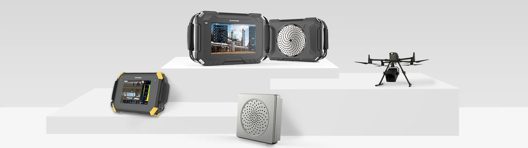
Acoustic cameras turn invisible sound into visible images. This guide explains how they work, where they're used, and how to choose the right one for your application. What Is an Acoustic Camera? An acoustic camera is a device that locates and visualizes sound sources in real time. It combines a microphone array — typically 64 to 200+ MEMS microphones arranged in a specific pattern — with a video camera and signal processing software. The result is a color-coded overlay on a live video feed, showing exactly where sound is coming from and how loud it is. Think of it as a thermal camera, but for sound instead of heat. Where a thermal camera shows hot spots in red, an acoustic camera shows loud spots — pinpointing the exact location of a leak, a faulty bearing, or an electrical discharge that you can't see with your eyes. The technology was originally developed for aerospace and automotive NVH (Noise, Vibration, and Harshness) testing. Today, it has expanded into industrial maintenance, energy utilities, manufacturing quality control, and building acoustics. How Does an Acoustic Camera Work? How an acoustic camera uses beamforming: sound waves arrive at each microphone with different time delays (Δt), the processor combines all signals, and outputs a color-coded sound map. The Microphone Array At the core of every acoustic camera is a microphone array — a precisely arranged set of MEMS (Micro-Electro-Mechanical Systems) microphones. The number of microphones directly affects performance: 64 microphones: Entry-level, suitable for general-purpose sound source localization 128 microphones: Professional-grade, better resolution and dynamic range 200+ microphones: High-end, capable of detecting subtle sources in noisy environments The spatial arrangement of these microphones matters as much as the count. Common configurations include circular, spiral (Fibonacci), and grid patterns. Each has trade-offs: spiral arrays offer good broadband performance, while grid arrays are better for near-field measurements. Beamforming: The Core Algorithm The key technology behind acoustic cameras is beamforming — a signal processing technique that combines signals from multiple microphones to "focus" on specific locations in space. Here's a simplified explanation: A sound wave arrives at each microphone at slightly different times (because each microphone is at a different distance from the source) The software calculates the expected time delay for every possible source location in the field of view For each candidate location, it shifts and sums the microphone signals according to the calculated delays Locations where the shifted signals add up constructively are identified as sound sources This process is repeated for every pixel in the image, producing a "sound map" that shows the spatial distribution of sound energy. Beamforming vs. Acoustic Holography There are two main acoustic imaging technologies: FeatureBeamformingAcoustic Holography (NAH)Best frequency rangeMid to high frequencies (>500 Hz)Low frequencies (<2 kHz)Measurement distanceFar-field (>1 meter)Near-field (<30 cm from source)ResolutionLimited by wavelength and array sizeHigher resolution at low frequenciesSpeedReal-time capableRequires careful scanningBest forLeak detection, general noise mappingEngine NVH, vibration analysis Most modern acoustic cameras use beamforming as the primary method because it works in real time and doesn't require the camera to be positioned close to the source. Some advanced systems support both technologies for maximum flexibility. The Role of the Video Camera The microphone array generates a sound map; the video camera provides the visual reference. The software overlays the sound map onto the video feed as a color-coded heat map, allowing the user to instantly see which component, pipe, or connection is producing the sound. High-end systems use depth cameras (such as Intel RealSense) to create 3D acoustic maps, enabling more accurate source localization on complex geometry. Frequency Range: Why It Matters Different applications require different frequency ranges: ApplicationTypical Frequency RangeWhyCompressed air leak detection20–50 kHzLeaks produce high-frequency hissingPartial discharge detection20–100 kHzElectrical discharges emit ultrasonic signalsMechanical fault detection1–20 kHzBearing wear, misalignment produce audible noiseAutomotive NVH100 Hz–10 kHzRoad noise, wind noise, engine noiseBuilding acoustics50 Hz–8 kHzLow-frequency structure-borne noise An acoustic camera with a frequency range of up to 100 kHz can handle virtually all industrial applications, including ultrasonic leak and partial discharge detection. Cameras limited to 20 kHz are suitable only for audible noise analysis. Key Applications Acoustic camera detecting vacuum leaks in composite materials — the color overlay pinpoints the exact leak location on the surface. Partial discharge detection on high-voltage insulators — the acoustic camera identifies discharge locations from a safe distance, combined with infrared thermal imaging for comprehensive diagnostics. 1. Compressed Air Leak Detection Compressed air is one of the most expensive energy sources in a factory. Studies show that 20–30% of compressed air is lost to leaks. An acoustic camera can scan an entire production line in minutes, identifying leaks that are invisible and inaudible to human ears. Why acoustic cameras beat traditional methods: Ultrasonic leak detectors require you to check one point at a time; an acoustic camera scans an entire area at once Visual overlay pinpoints the exact location — no guessing Many systems can estimate leak rate and annual cost, helping you prioritize repairs 2. Electrical Partial Discharge Detection Partial discharge (PD) is an early warning sign of insulation failure in high-voltage equipment — transformers, switchgear, cables, and bus bars. Left undetected, PD leads to complete insulation breakdown and potentially catastrophic failure. Acoustic cameras detect PD by capturing the ultrasonic emissions (typically 20–100 kHz) that accompany electrical discharge. The advantage over traditional PD detection methods: Non-contact: No need to de-energize equipment Real-time visualization: See exactly where the discharge is occurring Safe distance: Inspect live equipment from several meters away 3. Mechanical Fault Diagnosis Worn bearings, misaligned shafts, loose components, and valve leaks all produce characteristic sound signatures. An acoustic camera can identify and locate these faults before they lead to unplanned downtime. Common use cases: Motor and pump bearing wear detection Steam trap malfunction Valve leak identification Gearbox noise analysis 4. Automotive and Aerospace NVH Testing This is where acoustic cameras originated. NVH engineers use them to: Identify wind noise sources on vehicle bodies Locate rattles and squeaks in interior trim Analyze tire/road noise contributions Map engine noise radiation patterns Validate sound package effectiveness For NVH applications, large-aperture arrays (200+ microphones) provide the resolution needed to distinguish closely spaced sources. 5. Noise Compliance and Building Acoustics Environmental noise regulations require manufacturers to identify and reduce noise emissions. Acoustic cameras help: Map factory noise sources for compliance reporting Identify noise paths in buildings (walls, windows, HVAC) Verify effectiveness of noise barriers and enclosures 6. UAV-Mounted Acoustic Inspection A newer application: mounting acoustic cameras on drones for inspection of hard-to-reach infrastructure. Applications include: Power line and substation inspection Wind turbine blade inspection Pipeline corridor leak surveys Tall structure noise mapping Types of Acoustic Cameras Four form factors of acoustic cameras: Handheld (CRY8124), Fixed-Mount (CRY2623M), Large Array (CRY8500 SonoCAM Pi), and UAV-Mounted (CRY2626G). Handheld Acoustic Cameras Portable, battery-powered devices for field use. Typically 64–128 microphones with a built-in display. Best for maintenance rounds, leak detection, and quick inspections. Pros: Portable, easy to use, quick deployment Cons: Limited microphone count, smaller array = lower resolution at distance Fixed/Mounted Acoustic Cameras Permanently installed for continuous monitoring. Used in power substations, data centers, and critical infrastructure. Can run 24/7 with automated alerts. Pros: Continuous monitoring, automated alerting, no operator needed Cons: Fixed field of view, higher installation cost Large-Array Systems 200+ microphones on a larger frame. Used for NVH testing, pass-by noise measurement, and research applications. Often mounted on tripods or overhead structures. Pros: Highest resolution, widest frequency range, best for complex analysis Cons: Not portable, requires setup, higher cost UAV-Mounted Systems Lightweight acoustic arrays designed for drone mounting. Used for remote inspection of power lines, pipelines, and industrial facilities. Pros: Access to hard-to-reach locations, large-area surveys Cons: Flight time limits, vibration interference, regulatory requirements How to Choose the Right Acoustic Camera Quick decision guide: Choose your acoustic camera based on primary application. Step 1: Define Your Primary Application Your application determines the minimum specifications: ApplicationMin. MicrophonesFrequency RangeForm FactorCompressed air leak detection64Up to 50 kHzHandheldPartial discharge detection64–128Up to 100 kHzHandheld or fixedMechanical fault diagnosis64Up to 20 kHzHandheldNVH testing128–200+100 Hz–20 kHzLarge arrayContinuous monitoring64–128Application-dependentFixedDrone inspection64–128Up to 50 kHzUAV-mounted Step 2: Consider the Environment Noisy factory floor? You need more microphones and advanced algorithms to separate the target signal from background noise Outdoor use? Look for weather-resistant designs and wind noise rejection Hazardous area? Check for ATEX/IECEx certification Large distance? More microphones = better resolution at range Step 3: Evaluate the Software The hardware captures the data; the software turns it into actionable information. Key software features to look for: Real-time display: See the sound map live as you scan Frequency filtering: Isolate specific frequency bands to focus on particular issues Leak rate estimation: Quantify the cost of leaks in dollars or energy units Reporting: Generate professional reports with screenshots, measurements, and recommendations AI-assisted detection: Automatic identification of leak patterns and fault signatures Step 4: Compare Specifications Key specs to compare across manufacturers: SpecificationWhat It MeansWhat to Look ForMicrophone countMore mics = better resolution and sensitivity64 minimum; 128+ for demanding applicationsFrequency rangeDetermines what you can detectUp to 100 kHz for PD and ultrasonic leaksDynamic rangeAbility to measure both quiet and loud sources>70 dB for industrial environmentsAngular resolutionAbility to separate nearby sourcesSmaller is better; depends on frequency and distanceFrame rateHow quickly the sound map updates>10 fps for real-time scanningWeight and sizePortability<2 kg for handheld daily-use devicesBattery lifeRuntime for field use>3 hours for a full shift of inspectionsIP ratingDust and water resistanceIP54 or higher for industrial environments CRYSOUND Acoustic Camera Solutions CRYSOUND offers one of the widest product lines in the acoustic camera market — covering handheld, fixed-mount, large-array, and UAV-mounted form factors from a single manufacturer. Product Lineup CRY2624: 128-microphone handheld acoustic camera with ATEX certification — portable, field-ready, and safe for hazardous environments CRY8124: 200 MEMS microphones, frequency range up to 100 kHz — handles both audible noise analysis and ultrasonic applications (leak detection + partial discharge) in a single device CRY2623M: Fixed-mount version for 24/7 continuous monitoring of substations and critical infrastructure CRY8500 Series (SonoCAM Pi): Large spiral microphone array for NVH testing, pass-by noise measurement, and advanced acoustic research CRY2626G: Drone-mounted acoustic camera for remote inspection of power lines, pipelines, and wind turbines CRYSOUND acoustic camera product family: from handheld to drone-mounted solutions. Key Differentiator 1: Modular Sensor Expansion Unlike most competitors that offer a fixed-function device, CRYSOUND's acoustic cameras support external sensor modules for expanded capabilities: Infrared thermal imaging module: Combines acoustic and thermal data in a single view — when inspecting power equipment, engineers can simultaneously see the acoustic signature of partial discharge and the thermal hot spot of overheating components. This dual-mode inspection is widely used in power utilities for comprehensive substation diagnostics. IA3104 Contact Ultrasound Sensor: An external contact-type ultrasonic probe designed specifically for valve internal leak detection. The sensor couples directly to the metal surface of a valve, capturing high-frequency ultrasonic signals generated by internal leakage. Combined with intelligent analytics and guided workflows, it automates the full diagnostic process — from data acquisition to leak classification. This is critical for preventive maintenance of oil pipeline valves and natural gas network valves. This modular approach means a single CRYSOUND acoustic camera can serve as a comprehensive inspection platform, rather than requiring separate instruments for each detection task. Key Differentiator 2: Acoustic Link Mobile App CRYSOUND's Acoustic Link is a companion mobile app that connects to the acoustic camera via Wi-Fi. It enables: On-device preview: View captured photos, videos, and inspection reports on your phone or tablet — no PC required Defect-specific visualization: Retrieve gas-leak acoustic maps, partial-discharge patterns, and thermal images directly in the app One-tap sharing: Save results locally and share via the system share sheet for instant communication with colleagues and customers Automated report generation: Generate and export professional inspection reports from the field, eliminating the need to return to the office for post-processing For field inspection teams, this means faster turnaround from detection to documentation. Key Differentiator 3: Complete Acoustic Ecosystem Beyond acoustic cameras, CRYSOUND manufactures electroacoustic test systems (CRY6151B), acoustic test chambers, and calibration equipment — enabling complete acoustic testing solutions from a single vendor. With 28 years of experience and over 10,000 customers across 90+ countries, CRYSOUND brings deep domain expertise to every product. Explore CRYSOUND Acoustic Camera Products → Frequently Asked Questions What is the difference between an acoustic camera and a sound level meter? A sound level meter measures the overall sound pressure level at a single point. It tells you how loud it is, but not where the sound comes from. An acoustic camera shows both the location and the intensity of sound sources, making it far more useful for diagnosing and fixing noise problems. How far away can an acoustic camera detect a leak? Detection range depends on the leak size, background noise, microphone count, and frequency range. A typical handheld acoustic camera with 64–128 microphones can detect a 1mm compressed air leak from 10–30 meters away. Larger leaks can be detected from even greater distances. Can an acoustic camera work in a noisy factory? Yes. Modern acoustic cameras use beamforming algorithms that can isolate specific sound sources even in high-background-noise environments. The key is having enough microphones — more microphones provide better noise rejection and higher signal-to-noise ratio. Do I need training to use an acoustic camera? Basic operation is straightforward — point the camera, look at the screen, and identify the highlighted areas. Most users can start finding leaks within minutes. However, interpreting complex acoustic patterns (NVH analysis, partial discharge classification) benefits from training and experience. What is the ROI of an acoustic camera? For compressed air leak detection alone, the ROI is typically measured in months. A single quarter-inch air leak costs $2,500–$8,000 per year. Most industrial facilities have dozens to hundreds of leaks. An acoustic camera that helps you find and fix these leaks can pay for itself in the first survey. Can acoustic cameras detect gas leaks other than compressed air? Yes. Acoustic cameras can detect any pressurized gas leak that produces turbulent flow noise — including nitrogen, oxygen, hydrogen, natural gas, and refrigerants. The frequency characteristics may vary by gas type, but the detection principle is the same. Need help choosing the right acoustic camera for your application? Contact CRYSOUND for a personalized recommendation based on your specific requirements.
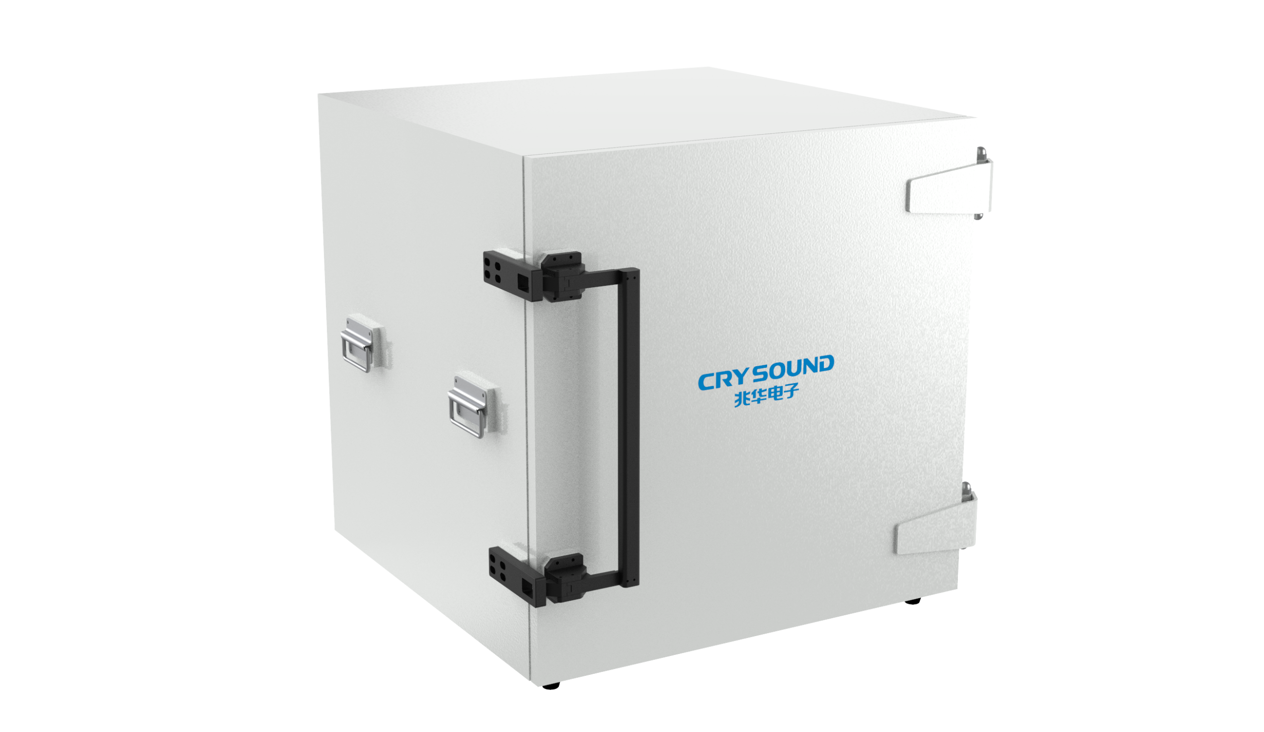
Why Choosing the Right Acoustic Test Chamber Matters In electroacoustic testing and wireless device production, the test chamber is not just a box — it directly affects measurement accuracy, throughput, and production costs. The wrong chamber can introduce background noise into your measurements, fail to shield RF interference, or simply not fit your DUT (Device Under Test). This guide walks you through the key factors for selecting an acoustic test chamber, with a comparison of CRYSOUND’s product range to help you match the right model to your application. Key Selection Criteria 1. What Are You Testing? The size and type of your DUT is the first deciding factor: DUT TypeTypical ProductsChamber RequirementSmall wireless devicesTWS earbuds, smartphones, smart watchesCompact chamber with RF shieldingMedium devicesBluetooth speakers, headphones, smart home devicesMid-size chamber with good low-frequency isolationLarge devicesLaptops, walkie-talkies, wireless serversLarge chamber with full RF shieldingUltra-quiet testingMEMS microphones, hearing aids, high-sensitivity sensorsUltra-low noise floor chamber 2. Acoustic Isolation Performance How much noise do you need to block? If your production floor is noisy (70–80 dB ambient), you need a chamber with high sound attenuation to achieve a clean measurement environment. For laboratory settings that are already relatively quiet, a lighter chamber may suffice. Key spec to check: Sound attenuation (dB) across the frequency range relevant to your product. Pay special attention to low-frequency attenuation — this is where most chambers struggle, and where the CRY725D specifically excels. 3. RF Shielding If you are testing wireless devices (Bluetooth, WiFi, GSM, WCDMA, RFID, GPS), RF shielding is essential to prevent interference between adjacent production lines. Without it, neighbouring test stations can cause false failures. Key spec to check: Shielding effectiveness (dB) at the frequencies your device operates on. 4. Door Mechanism: Pneumatic vs Manual FeaturePneumatic DoorManual DoorSpeedFast open/close, ideal for high-volume productionSlower, suitable for lab or low-volumeAutomationSerial port / PLC control, integrates into automated linesManual operation onlyConsistencyRepeatable sealing force every cycleDepends on operatorCostHigher (requires air supply)LowerBest forProduction linesR&D labs, occasional testing 5. Production Line Integration For high-volume manufacturing, consider: Drawer-style design — slides into automated test racks (e.g. CRY7865, CRY725D) Shell-type design — pairs with analysers for multi-station operation (e.g. CRY723) Serial port control — enables software-triggered open/close for fully automated test sequences CRYSOUND Acoustic Test Chamber Lineup Here is a comparison of our full product range, organised by application scenario: For Smartphones & Wireless Wearables CRY723 Pneumatic Acoustic Test Chamber Design: Shell-type, compact form factor Best for: Smartphones, TWS earbuds, smart watches, wireless wearables Key advantage: Cost-effective and high-performance. Combine two CRY723 units with a CRY6151B analyser for complete audio, ENC, and ANC measurements — one operator manages two test stations simultaneously Door: Pneumatic CRY723D Pneumatic Acoustic Test Chamber Design: Enhanced version of CRY723 Best for: Wireless electronic and communication products requiring comprehensive RF testing Key advantage: Full wireless connectivity support — Bluetooth, WiFi, GSM, WCDMA, RFID, GPS Door: Pneumatic For Large Wireless Devices CRY725 Pneumatic Acoustic Test Chamber Design: Large-format chamber Best for: Laptops, walkie-talkies, wireless servers, and other large wireless devices Key advantage: Spacious internal volume for large DUTs, compatible with comprehensive testers and vector network analysers Door: Pneumatic CRY725D Pneumatic Acoustic Test Chamber Design: Drawer-style, enhanced low-frequency performance Best for: Background noise measurement, applications requiring superior low-frequency isolation Key advantage: Superior soundproofing at low frequencies compared to CRY725. Combined with CRY6151B and CRY algorithm, provides enhanced noise floor minimisation for precision testing Door: Pneumatic (drawer-style) For Production Line Integration CRY7865 Pneumatic Acoustic Test Chamber Design: Drawer-style, designed for rack integration Best for: Automated production lines testing Bluetooth headphones, speakers, laptops Key advantage: High-performance acoustic isolation and RF shielding in one unit. Drawer-style design facilitates seamless integration into automated test systems Door: Pneumatic (drawer) CRY710 Pneumatic Acoustic Test Chamber Design: Welded steel plate construction, robust RF shielding Best for: Bluetooth, WiFi device testing where strong RF shielding is the priority Key advantage: Prevents interference between adjacent production lines. Combine two CRY710 units with a CRY6151B for quadruplex TWS headphone audio testing Door: Pneumatic (serial port controlled) For R&D and Laboratory Use CRY7413 Acoustic Test Chamber, Manual Door Design: Compact, manual door, adjustable test jig Best for: R&D labs, product development, low-volume testing Key advantage: User-friendly design with marked and adjustable test jig that accommodates various DUT sizes. Quick DUT exchange with minimal operator strain Door: Manual CRY7412 Ultra-Quiet Chamber Design: Double-shell (box-in-box), lateral two-stage opening Best for: Testing very quiet sounds — MEMS microphones, hearing aids, high-sensitivity sensors Key advantage: Unique box-in-box design provides the lowest noise floor in the product range. Essential when your DUT produces very low sound levels that would be masked by ambient noise in a standard chamber Door: Manual (two-stage lateral opening) Quick Selection Guide Your SituationRecommended ModelWhyTesting TWS earbuds on a production lineCRY723Compact, cost-effective, dual-station with CRY6151BTesting laptops or large wireless devicesCRY725Large internal volume, full RF shieldingNeed superior low-frequency isolationCRY725DEnhanced low-frequency soundproofingAutomated production line integrationCRY7865Drawer-style, RF + acoustic shieldingBluetooth/WiFi RF isolation is priorityCRY710Robust welded steel RF shieldingR&D lab, various DUT sizesCRY7413Adjustable jig, easy DUT exchangeMeasuring very quiet soundsCRY7412Double-shell, lowest noise floor Frequently Asked Questions Do I need RF shielding in my acoustic test chamber? If you are testing any wireless device (Bluetooth, WiFi, cellular), the answer is yes. Without RF shielding, wireless signals from neighbouring test stations or production equipment can cause false test failures. All CRYSOUND pneumatic chambers include RF shielding as standard. Can I use one chamber for both R&D and production? Yes, but the optimal choice differs. For R&D, flexibility and low noise floor matter most (CRY7413 or CRY7412). For production, speed and automation matter most (CRY723, CRY7865). If you need both, consider the CRY723 — it balances performance, automation capability, and cost. What is the advantage of drawer-style vs shell-type chambers? Drawer-style (CRY7865, CRY725D) slides into standard equipment racks and integrates cleanly into automated test lines. Shell-type (CRY723) opens like a clamshell for quick DUT loading and is more versatile for varied DUT shapes. Choose drawer-style for fixed production setups; shell-type for flexible or multi-product lines. How do I reduce labour costs in acoustic testing? Combine two test chambers with a single CRY6151B electroacoustic analyser. While one DUT is being tested, the operator loads the next DUT in the second chamber. This dual-station setup — supported by CRY723, CRY710, and other models — effectively doubles throughput with no additional headcount. Need Help Choosing? Every production environment is different. If you are unsure which model fits your requirements, our engineering team can help you evaluate your testing needs and recommend the right configuration. Contact CRYSOUND for a personalised recommendation based on your DUT, production volume, and test requirements.
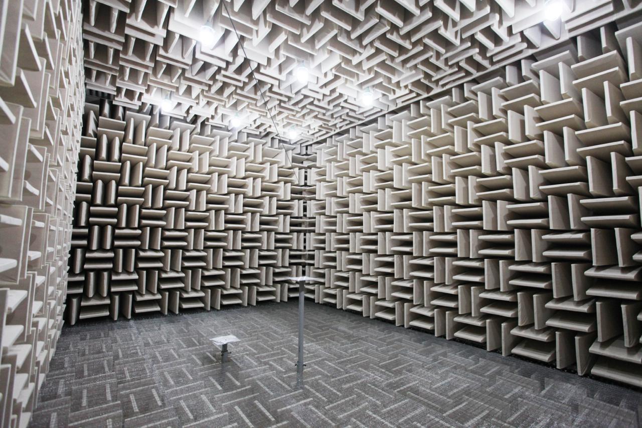
What Is an Anechoic Chamber? An anechoic chamber is a room designed to completely absorb sound reflections. The walls, ceiling, and (in a full anechoic chamber) the floor are lined with wedge-shaped foam or fibreglass absorbers that prevent sound waves from bouncing back into the room. The result is a controlled acoustic environment that simulates free-field conditions — as if the sound source were suspended in open air with no surfaces nearby. This matters because most acoustic measurements — sound power, directivity, frequency response — require a known, reflection-free environment to produce repeatable, standards-compliant results. Without it, room reflections contaminate the measurement, making results dependent on the specific room rather than the product being tested. Full Anechoic vs Semi-Anechoic (Hemi-Anechoic) Chambers Feature Full Anechoic Semi-Anechoic (Hemi-Anechoic) Absorbing surfaces All 6 surfaces (walls, ceiling, floor) 5 surfaces (walls + ceiling); floor is reflective Floor Wire mesh or perforated metal grid suspended above absorbers Solid, load-bearing concrete or steel Acoustic condition Free-field (no reflections from any direction) Free-field over a reflecting plane Load capacity Limited — cannot support heavy equipment directly Can support vehicles, machinery, industrial equipment Primary standards ISO 3745 (precision sound power) ISO 3744 (engineering sound power), ISO 3745 Typical use Microphone calibration, loudspeaker characterisation, hearing research Automotive NVH, product noise testing, industrial machinery Cost Higher (floor treatment adds significant cost and complexity) Lower (no floor treatment needed) In practice, about 80% of industrial acoustic testing uses semi-anechoic chambers because most test objects — cars, appliances, compressors, power tools — are too heavy for a suspended wire-mesh floor. What Standards Require an Anechoic Chamber? ISO 3745 — Precision Sound Power Measurement The gold standard for sound power determination. Requires either a full anechoic or hemi-anechoic chamber qualified to meet strict free-field deviation limits across the frequency range of interest. The chamber must demonstrate that the inverse-square law holds to within ±1 dB at the measurement positions. Typical cut-off frequency: 80–200 Hz, depending on chamber size and wedge depth. Below this frequency, the chamber no longer behaves as a free field. ISO 3744 — Engineering Sound Power Measurement Less stringent than ISO 3745 but still requires a hemi-anechoic environment. Allows for environmental corrections when the room is not perfectly anechoic, making it practical for production-floor test cells that approximate (but do not perfectly achieve) free-field conditions. ISO 26101 — Qualification of Free-Field Environments Defines how to verify whether a room actually meets free-field requirements. This is the standard used to “qualify” an anechoic or hemi-anechoic chamber — confirming that its acoustic performance matches what is claimed. Other Standards ECMA-74: IT equipment noise measurement (uses ISO 3745 or ISO 3744 as the underlying acoustic method) ANSI S12.55 / S12.56: North American equivalents of ISO 3744/3745 ISO 11201–11205: Various sound pressure level determination methods, some requiring free-field conditions Key Design Considerations 1. Chamber Size and Usable Volume The physical dimensions determine the lowest usable frequency. A general rule: the chamber must be large enough that the distance between the sound source and each measurement microphone is at least one wavelength at the lowest frequency of interest. For a 100 Hz cut-off, the minimum source-to-microphone distance is approximately 3.4 metres, which means the chamber’s internal dimensions (excluding wedges) should be at least 7–8 metres per side for a hemi-anechoic chamber. 2. Wedge Absorbers The depth of the absorbing wedges determines the low-frequency performance. Deeper wedges absorb lower frequencies: Wedge Depth Approximate Low-Frequency Cut-off 200 mm ~500 Hz 500 mm ~200 Hz 1000 mm ~80–100 Hz Wedge materials include melamine foam (lightweight, fire-retardant) and fibreglass (better low-frequency absorption but heavier). 3. Background Noise An anechoic chamber must also be well-isolated from external noise. The ambient noise level inside the chamber (with no source operating) should be at least 6 dB — and preferably 15 dB — below the sound pressure level generated by the test object at the measurement positions. This typically requires a chamber built with multiple layers of massive construction (concrete, steel) and vibration-isolated mounting to prevent structure-borne noise transmission. 4. Vibration Isolation For NVH testing (especially automotive), the chamber floor may include vibration-isolated foundations or air-spring mounting systems to prevent road-simulator or dynamometer vibrations from coupling into the acoustic measurement environment. What If You Do Not Have an Anechoic Chamber? Not every organisation can invest $500K–$2M+ in a purpose-built anechoic facility. Several practical alternatives exist: Sound Intensity Method (ISO 9614) Sound intensity measurements are inherently less sensitive to room reflections because intensity is a vector quantity — it distinguishes between outgoing sound (from the source) and incoming sound (reflections from room surfaces). This allows sound power determination in ordinary rooms without anechoic treatment. Trade-off: Requires specialised intensity probes and more complex measurement procedures. Acoustic Test Boxes For small products (electronics, components, transducers), a desktop-sized acoustic test box provides a controlled, low-noise environment that approximates anechoic conditions within a defined frequency range. These are significantly cheaper than a full chamber and can be placed directly on a production line. CRYSOUND offers a comprehensive range of acoustic test chambers designed for different testing scenarios: CRY723 Pneumatic Acoustic Test Chamber — A compact, shell-type test box ideal for smartphones and wireless wearables. Combine two CRY723 units with a CRY6151B analyzer for complete audio, ENC, and ANC measurements. CRY725 Pneumatic Acoustic Test Chamber — Designed for larger wireless devices such as laptops and walkie-talkies. Compatible with comprehensive testers and vector network analyzers. CRY7865 Pneumatic Acoustic Test Chamber — A high-performance drawer-style chamber with both acoustic isolation and RF shielding, ideal for production line audio and noise measurements of wireless electronic devices. CRY7412 Ultra-Quiet Chamber — An ultra-quiet chamber for testing very quiet sounds in noisy environments. Features a unique double-shell design for superior noise isolation. All models support pneumatic operation for fast, repeatable DUT loading on production lines — a practical alternative when a full anechoic chamber is not justified by the application. Portable Acoustic Arrays Modern acoustic imaging cameras can identify and localise noise sources in situ — in the factory, on the production line, or in the field — without any anechoic treatment. While not a substitute for standards-compliant sound power measurements, acoustic imaging enables rapid noise source diagnosis that previously required dedicated chamber time. The CRY8500 Series SonoCam Pi Acoustic Camera, is a portable acoustic imaging camera that delivers real-time sound source visualisation — ideal for R&D engineers working on noise source identification in automotive NVH, industrial equipment, and consumer electronics. In-Situ Sound Power (ISO 3744 with Corrections) ISO 3744 allows environmental correction factors to account for room reflections. If the correction is small (typically less than 2 dB), the measurement can be performed in a reasonably quiet industrial space without a purpose-built chamber. The SonoDAQ Pro data acquisition system combined with OpenTest software supports automated sound power calculations with environmental corrections built in — enabling standards-compliant measurements without a dedicated anechoic chamber. Frequently Asked Questions How much does an anechoic chamber cost? Costs vary widely based on size, performance requirements, and cut-off frequency. A small hemi-anechoic room for component testing may start around $100K–$300K, while a large automotive-grade full anechoic chamber can exceed $2M. For smaller products, acoustic test boxes offer similar isolation at a fraction of the cost. What is the difference between an anechoic chamber and a soundproof room? A soundproof room blocks external noise from entering but does nothing about internal reflections. An anechoic chamber both blocks external noise and absorbs internal reflections, creating a free-field environment for precision measurement. Can I do acoustic testing without an anechoic chamber? Yes. Depending on your application, alternatives include acoustic test boxes for small products, sound intensity methods (ISO 9614), portable acoustic imaging cameras like the CRY8500 SonoCam Pi, and in-situ measurements with environmental corrections using systems like SonoDAQ Pro. What frequency range does an anechoic chamber cover? The usable frequency range depends on the wedge depth and chamber dimensions. Most chambers are effective from their cut-off frequency (typically 80–200 Hz) up to 20 kHz or beyond. Below the cut-off, the chamber no longer provides adequate absorption. How is an anechoic chamber qualified? Chamber qualification follows ISO 26101, which verifies that the inverse-square law (sound pressure decreasing by 6 dB per doubling of distance) holds within specified tolerances at the measurement positions. Conclusion Anechoic chambers remain the gold standard for precision acoustic measurement — but they are not the only option. Understanding what your application truly requires helps you choose the right solution, whether that is a full anechoic room, a compact acoustic test chamber, or an in-situ measurement approach. At CRYSOUND, we provide the full spectrum: from purpose-built anechoic chambers to portable acoustic test boxes and advanced measurement systems — so you can get accurate results regardless of your facility constraints. Contact us to discuss which solution fits your testing requirements.

During pilot production and production line ramp-up, many issues do not appear in the way teams initially expect. Sometimes it starts with a small fluctuation at a test station, or a comment from a line engineer saying, "This result looks a bit unusual."However, when takt time, yield targets, and delivery milestones are all under pressure, these seemingly minor anomalies can quickly be amplified and begin to affect the overall production rhythm. We have been working with Huaqin as a long-term partner. As projects progressed, the challenges encountered on the production line became increasingly complex. On site, our role gradually extended from basic production test support to problem analysis and cross-team coordination during pilot production. In many cases, the focus was not simply on whether a test station was functioning, but on how to absorb uncertainties early and prevent them from disrupting delivery schedules. The following two experiences both took place during the pilot production phase of Huaqin projects. They are not exceptional cases. On the contrary, they represent the kind of everyday issues that most accurately reflect the realities of production line delivery. Airtightness Testing Issues in Project α During the pilot ramp-up of Project α, the airtightness test station for the audio microphone showed clear instability. For the same batch of products, pass rates fluctuated noticeably across repeated tests, frequently interrupting the station's operating rhythm. Initial troubleshooting naturally focused on the test system itself, including software logic, equipment status, and basic parameter settings. It soon became clear, however, that the issue did not originate from these areas. As on-site verification continued, we gradually confirmed that the anomaly was more closely related to the product's mechanical structure and material characteristics. This model used a relatively uncommon combination of materials. A sealing solution that had worked well in previous projects could not maintain consistency during actual compression. Even slight variations in applied pressure were enough to influence test results. Once the direction of the problem was clarified, the on-site approach shifted accordingly. Rather than repeatedly adjusting the existing solution, we returned to verifying the compatibility between materials and structure. Over the following period, we worked together with the customer's engineering team on the production line, testing multiple material options. This included different types of silicone and cushioning materials, variations in silicone hardness, and adjustments to plug compression methods. Each step was evaluated based on real test results before moving forward. The process was not fast, nor was it particularly clever. In essence, it came down to repeatedly confirming one question: could this solution run stably under real production line conditions?Ultimately, by introducing a customized soft silicone gasket and making fine parameter adjustments, the airtightness test results gradually stabilized. The station was able to run continuously, and the pilot production rhythm was restored. Figure 1. Test Fixture Diagram Noise Floor Issues in Project β Compared with the airtightness issue in Project α, the noise floor anomaly encountered during pilot production in Project β was more complex to diagnose. During headphone pilot production for Project β at Huaqin's Nanchang site, the noise floor test station repeatedly triggered alarms. Test data showed that measured noise levels consistently exceeded specification limits, significantly impacting the pilot production schedule. This model used high-sensitivity drivers along with a new circuit design, making the potential noise sources inherently more complex. It was not a problem that could be resolved by simply adjusting a single parameter. Rather than focusing solely on the test station, we worked with the customer's audio team to investigate the issue from a system-level signal chain perspective. The process involved sequentially testing different shielding cables, adjusting grounding strategies, evaluating various Bluetooth dongle connection methods, and isolating potential power supply and electromagnetic interference sources within the test environment. Through continuous spectrum analysis and comparative testing, the scope of the issue was gradually narrowed. It was ultimately confirmed that the elevated noise floor was primarily related to power interference from the Bluetooth dongle, combined with differences in product behavior across operating states. After this conclusion was reached, relevant configurations were adjusted and validated on site. As a result, noise floor measurements returned to a stable and controllable range, allowing pilot production to proceed. Figure 2. Work with the customer engineer to solve problems Common Characteristics of Pilot Production Issues Looking back at these two pilot production experiences, it becomes clear that despite their different manifestations, the underlying diagnostic processes were quite similar. Whether dealing with airtightness instability or excessive noise, the root cause could not be isolated to a single module. Effective resolution required on-site evaluation across mechanical structure, materials, system operating states, and test conditions. During pilot production, issues of this nature rarely come with ready-made answers. They are also unlikely to be resolved through a single verification cycle. More often, progress is made through repeated trials, comparisons, and eliminations, gradually converging on a solution that is genuinely suitable for long-term production line operation. Production line delivery rarely follows a perfectly smooth path. In many cases, what ultimately determines whether a project can move forward as planned are those unexpected issues that must be addressed immediately when they arise. In our long-term collaboration with customers, our work often takes place at these critical moments—working alongside engineering teams to stabilize processes, maintain momentum, and keep projects moving forward step by step. If you also want CRYSOUND to support your production line, you can fill out the Get in Touch form below.


