Blogs

Banner image for False Positives in Acoustic Imaging blog post featuring CRY8124 camera and diagnostic workflow

Acoustic Imaging False Positives: Reflections, Beamforming Artifacts, and How to Avoid Them

You're scanning overhead pipework in a compressor room when your acoustic camera shows a bright hotspot on a steel support beam. You walk over, listen carefully, and check the surface. Nothing. No hiss, no vibration, no leak. The image looks convincing, but the source is not actually on that beam. This is one of the most common acoustic imaging false positives engineers see in the field. Acoustic camera reflections, beamforming artifacts, and background noise can all create ghost images or false hotspots that look like real leaks, discharges, or mechanical faults. That does not mean the camera is malfunctioning. It means the operator needs to separate true sources from indirect paths and side responses. Based on field observations in reflective industrial environments, teams often find that 15–30% of initial acoustic indications should be treated as leads for verification rather than confirmed source locations. In this guide, we'll explain why an acoustic camera shows false hotspots, how to tell acoustic camera reflections from real leaks, and how to reduce beamforming artifacts in noisy factories without slowing down your inspection workflow. What Are False Positives in Acoustic Imaging? False positive (acoustic imaging): An apparent sound source indication on an acoustic camera display that does not correspond to an actual physical source at that location. Caused by physical phenomena including sound wave reflections, beamforming algorithm sidelobes, or environmental noise interference — not by equipment defect. Three related terms often get used interchangeably, but they describe different phenomena: False positive: Any indicated source that isn't real at the shown location Artifact: A systematic error pattern produced by the beamforming algorithm itself (e.g., sidelobes) Ghost image: A reflected or mirrored source — real sound arriving from an indirect path Understanding these distinctions matters because each type has different causes, different on-screen characteristics, and different solutions. Why Acoustic Cameras Show False Hotspots If your acoustic camera shows a hotspot on a wall, support beam, enclosure, or ceiling panel, the most common cause is a reflection rather than a leak at that exact surface. In other words, the hotspot may still be useful, but it is pointing to an indirect path instead of the true source location. If the display shows a halo, ring, or repeating spots around one strong source, that pattern is more likely a beamforming artifact than a second leak. And if the hotspot is broad, unstable, or spread across a noisy production area, environmental noise is usually a better explanation than a discrete defect. For teams using acoustic cameras in compressed air leak detection, it helps to pair this article with our acoustic camera guide and how acoustic imaging works explainer. If you need to quantify the cost of missed leaks before the next survey, use our air leak cost calculator. Common False Positives in Acoustic Cameras Reflections (Ghost Images) Sound waves bounce off hard, smooth surfaces — metal walls, concrete floors, glass panels, polished pipes — just like light reflects off a mirror. When your acoustic camera picks up both the direct sound and the reflected sound, the reflected path appears as a second source at a location where nothing is actually producing noise. Typical scenario: You're imaging a compressed air manifold mounted near a stainless steel wall. The display shows two hotspots — one on the manifold (real) and one on the wall behind it (ghost). The ghost image appears at roughly the same intensity and frequency as the real source. On-screen signature: Ghost images tend to appear at geometrically symmetrical positions relative to the reflecting surface. They share the same frequency spectrum as the real source and often appear at similar or slightly reduced intensity. Sidelobe Artifacts This is the most technically nuanced type. Beamforming algorithms work by mathematically "focusing" the microphone array on each point in the field of view. But just as a flashlight can't produce a perfectly sharp beam edge, beamforming produces a main lobe (the focused area) surrounded by sidelobes — weaker response regions that can register false sources. Typical scenario: You're imaging a single loud leak, but the display shows the main hotspot surrounded by a ring or pattern of secondary spots. These sidelobe artifacts are always clustered around the true source and become more pronounced when the source is loud relative to surrounding noise. On-screen signature: Sidelobes appear as a repeating pattern around the main source — often a ring, halo, or radial spoke pattern. Their intensity is always lower than the main lobe, and they maintain a fixed geometric relationship to the primary source regardless of scanning angle. Key factor: The number of microphone channels directly affects sidelobe levels. A 64-channel array produces more prominent sidelobes than a 128-channel array, which in turn produces more than a 200-channel array. Higher channel counts provide narrower main lobes and lower sidelobe floors. Advanced algorithms like CRYSOUND's HyperVision processing further suppress sidelobes beyond what standard delay-and-sum beamforming achieves. Environmental Noise Interference Not every unwanted indication is a reflection or algorithm artifact. Sometimes, your acoustic camera is accurately detecting a real sound — just not the one you're looking for. Background noise from HVAC systems, nearby machinery, overhead cranes, or even wind can register as apparent sources that get confused with your target. Typical scenario: During a compressed air leak survey in a manufacturing hall, you see multiple hotspots across a wide area. Some are genuine leaks. Others are background machinery noise that happens to fall within your selected frequency band. On-screen signature: Environmental noise sources typically have broader, more diffuse patterns than leaks (which appear as tight, focused hotspots). They also show different frequency characteristics — machinery noise tends to be narrower-band and harmonic, while leak noise is broadband and turbulent. Quick Comparison Type Cause On-Screen Signature Elimination Difficulty Reflections Sound bouncing off hard surfaces Symmetrical ghost image, same frequency as real source Moderate — multi-angle scan + frequency check Sidelobe artifacts Beamforming algorithm side response Ring/halo pattern around main source, lower intensity Low with advanced algorithms (HyperVision) Environmental noise Background machinery in frequency band Diffuse pattern, tonal/harmonic frequency profile Low — frequency filtering + Focus Function How to Identify False Positives: A 4-Step Process When you see an indication you're unsure about, run through these steps before logging it as a confirmed source: Angle change test. Move 2-3 meters to the side and re-scan the same area. Real sources stay in the same physical position on the image. Reflections shift or disappear as you change the angle of incidence. Sidelobes rotate with the main source. Frequency signature check. Switch to spectrum view (if your camera supports it) and examine the frequency profile. Compressed air leaks produce broadband, turbulent noise typically above 20 kHz. Machinery noise has distinct tonal peaks. If the "source" shares an identical spectrum with a known real source nearby, it's likely a reflection. Distance validation. If your camera allows distance-to-source measurement, check whether the indicated distance matches the physical geometry. A reflection off a wall 3 meters behind you will show a source distance that doesn't match the wall's position from your scanning location. Ultrasonic listening. Most acoustic cameras offer a downshift playback feature that converts the directionally-captured ultrasonic signal into audible sound through headphones. Point the camera at the suspect indication and listen. A real compressed air leak produces a distinctive broadband hiss. Sidelobe artifacts and reflections carry no independent acoustic signature — they sound identical to the main source. Environmental noise sounds tonal and harmonic. This lets you verify from your scanning position without walking to the indicated location. Techniques to Minimize False Positives 1. Select the Right Frequency Band Most acoustic cameras allow you to filter by frequency range. Narrowing the band to your target application reduces interference dramatically. For compressed air leaks, focus on 20–50 kHz. For partial discharge, 20–100 kHz. Excluding lower frequencies cuts out most machinery noise. 2. Use Advanced Beamforming Algorithms Not all beamforming is equal. Standard delay-and-sum (DAS) algorithms are computationally simple but produce higher sidelobe levels. Advanced algorithms apply spatial filtering to suppress sidelobes at the processing level. CRYSOUND's HyperVision algorithm, available on the CRY8124 and CRY8120 series, provides up to 10x processing power over standard beamforming, reducing sidelobe artifacts significantly without sacrificing real-time performance. 3. Adopt a Multi-Angle Scanning Protocol Make it standard practice to scan critical areas from at least two different positions. Compare the results. Sources that appear consistently in the same physical location are real. Sources that shift, disappear, or change intensity are false positives. This takes an extra 30 seconds per area and dramatically reduces misdiagnosis. Turning Artifacts into Allies: Using False Positives to Locate Sources Here's where experienced operators separate from beginners. False positives aren't just noise to eliminate — they carry information about the acoustic environment that you can exploit. Reflection Mapping If you see a ghost image on a metal wall, you've just learned something valuable: there's a real sound source at the geometrically mirrored position. The reflection tells you the sound wave's travel path. In complex piping environments where direct line-of-sight to a leak is blocked, reflected images on nearby surfaces can reveal the general direction and approximate distance of sources you can't see directly. Pro technique: When scanning in confined spaces with multiple reflective surfaces, intentionally note where ghost images appear. The pattern of reflections triangulates the true source location, even when the source is behind equipment or above a ceiling panel. Sidelobe Pattern Reading Sidelobes always radiate symmetrically from the main lobe. When you see a sidelobe pattern, the center of that pattern is your real source — guaranteed. In environments where obstructions partially block your view, the visible sidelobes can confirm the direction of a source that's partially hidden. If the sidelobe "ring" is only visible on one side, the true source is on the opposite side, behind whatever's blocking your view. Spatial Focusing (ROI Isolation) In noisy industrial environments, you can't shut down surrounding equipment just to get a cleaner acoustic image. Instead, use your camera's Focus Function: draw a region of interest (ROI) directly on the screen around the area you want to investigate. The camera restricts its beamforming analysis to that region only, effectively suppressing sound sources outside the selected area. This is particularly powerful when combined with frequency band filtering. Narrow the frequency range to your target application (e.g., 20–50 kHz for leak detection), then draw an ROI around the suspect zone. The double filter — spatial plus spectral — dramatically reduces environmental noise interference without requiring any change to the plant's operating conditions. What previously looked like a cluttered display with overlapping hotspots becomes a clean, focused view of the area that matters. Quick Reference Checklist Eliminating false positives: Set correct frequency band for target application Scan from at least two angles Check frequency spectrum of ambiguous sources Use ultrasonic listening to verify auditory signature before logging Leveraging false positives: Note reflection positions to triangulate hidden sources Read sidelobe patterns to confirm source direction Use Focus Function (ROI) to isolate target area from surrounding noise Need help diagnosing false positives? Talk to our application engineers → Frequently Asked Questions How common are false positives in acoustic imaging? Every acoustic camera produces some false positives. They are an inherent characteristic of beamforming physics, array geometry, and reflective environments rather than a product defect. With the right scanning workflow, most operators can tell a real source from a false hotspot within seconds. Why does my acoustic camera show a hotspot on the wall? The most common reason is reflection. The wall is acting like an acoustic mirror, so the camera detects indirect sound energy and maps it to the mirrored position. If the hotspot shifts or disappears when you change your scanning angle, you are likely looking at a reflection instead of a real source on that wall. What is the difference between a reflection and a beamforming artifact? A reflection is real sound reaching the array by an indirect path after bouncing off a surface. A beamforming artifact is a pattern generated by the imaging algorithm itself, often appearing as a halo or repeating side response around a strong source. Reflections usually move with geometry and angle; beamforming artifacts stay locked to the true source pattern. Can reflections be completely eliminated? No. As long as there are hard, smooth surfaces in the environment, sound will reflect. However, you can reduce their impact by scanning from multiple angles, matching spectra, and using region-of-interest controls to isolate the target area. Does a higher microphone channel count reduce artifacts? Yes. More channels generally provide a narrower main lobe and a lower sidelobe floor, which means fewer misleading side responses around strong sources. This is one reason acoustic camera specifications matter when you compare systems. How do I handle false positives in noisy factory environments? Use three filters together: narrow the frequency band to the target application, restrict the imaging area with an ROI or focus function, and confirm suspicious hotspots from a second angle. In most plants, that combination separates real leak-like sources from machinery noise fast enough for practical inspections. Can acoustic reflections actually help locate the real source? Yes. Reflections reveal the sound path, which means a ghost image can still tell you where to keep searching. In cluttered piping or enclosed machinery spaces, reflection patterns often help experienced operators triangulate the hidden source more quickly.

What Does "1000 V Isolation" Actually Isolate?

In many practical applications, data acquisition is not performed in an “ideal laboratory” environment. The device under test may be connected to mains power, distribution cabinets, frequency converters, or large electromechanical systems, while the acquisition card on the other side is connected via USB or Ethernet to a computer—sometimes operated directly by a person. These two sides are often not at the same electrical potential. If there is no effective electrical isolation inside the data acquisition card, this potential difference may propagate through signal lines, shields, or ground paths to the system side, leading to measurement distortion, interface malfunction, or even safety hazards. This is the fundamental reason why isolation exists in data acquisition systems. What Is the Isolation Rating of a Data Acquisition Card? In a data acquisition system, the isolation rating is not a simple voltage number, nor is it equivalent to “the voltage that the input can directly withstand.” It describes whether there is a reliable electrical isolation barrier between the measurement side (connected to sensors and the device under test) and the system side (connected to the host computer, communication interfaces, and power supply), and under what level of voltage stress this isolation remains valid. Isolation principle You can think of isolation as a bridge between two islands: The bridge allows information to pass—measurement data, digital communication, control signals. But it blocks dangerous currents—fault currents, ground-loop currents, and energy that could carry high potential to the host side. For this reason, isolation in data acquisition systems typically addresses both safety and measurement stability at the same time. Why Is Isolation Often More Important Than Accuracy Specifications? In many field applications, engineers do not encounter problems such as “insufficient resolution,” but instead: The same system works well in the lab, but noise increases dramatically on site. Once multiple devices are connected together, the data begins to drift. Replacing the computer or using a different power outlet suddenly makes the problem disappear. The common root cause behind these phenomena is often not algorithms or ADC performance, but rather improper handling of electrical potential relationships within the acquisition system. The value of isolation lies precisely here: by breaking unnecessary current loops and limiting the propagation paths of common-mode voltage and fault energy, isolation allows the acquisition system to behave in a controlled and predictable manner even in complex electrical environments. In industry discussions, the core values of isolation usually fall into three categories: signal integrity, safety, and instrument protection. Signal Integrity: Breaking Ground Loops and Improving Common-Mode Rejection Many cases of “inaccurate measurement” are not caused by ADC resolution, but by unwanted currents flowing through ground wires or shields. When the device under test and the host computer, enclosure, or other equipment are at different ground potentials, connecting them via signal cables may form ground loops. Power-line interference and electromagnetic noise then appear as “baseline noise” or ripple in the waveform. Isolation improves this by breaking the current loop paths. Safety: Confine High Potential and Fault Energy to the Measurement Side When measurement points are located near mains power, distribution cabinets, or frequency converters, the real risk is not merely “high voltage,” but where abnormal voltage or fault energy may propagate. If there is no clear electrical isolation between the measurement side and the host side, this energy may travel through signal or ground connections into the computer or communication interfaces, causing equipment damage or safety hazards. Isolation establishes a clear internal safety boundary: high potential and uncertain electrical environments are confined to the measurement side, while the system side—where the host computer and operator reside—remains within a controlled and safe potential range. If an abnormal condition occurs, the problem is contained on the measurement side and does not propagate further. Instrument Protection: A Larger Measurable Window Under High Common-Mode Voltage A non-isolated acquisition system effectively binds the measurement reference ground to system ground or earth. As a result, the measurable input range is centered around earth potential. If the entire signal shifts to a high common-mode potential, the front-end amplifier or ADC may exceed its allowable range or even be damaged. An isolated system allows the measurement reference to “float,” enabling the input measurement window to be centered around the isolated local ground. This permits operation under much higher common-mode voltages, with the ultimate limits determined by the isolation barrier and input protection circuitry together. Commonly Confused Isolation-Related Terms Isolation is often misunderstood because a single term—“isolation voltage”—is used to answer very different questions. The following clarifies these related but distinct concepts. Common-Mode Voltage Common-mode voltage refers to the voltage that is simultaneously applied to both measurement inputs relative to the acquisition system reference ground. It is not the signal of interest. The measurement signal concerns the difference between two input terminals, whereas common-mode voltage describes how high the two terminals are elevated together relative to ground. For example, in battery stacks or floating power systems, the signal itself may be only a few volts, but the entire source may be elevated tens or hundreds of volts above the acquisition card ground. In industrial environments, ground noise or electromagnetic interference may also impose time-varying AC voltage on both measurement leads. These “collectively elevated or oscillating voltages” constitute common-mode voltage. Working Voltage Working voltage is the voltage that can be continuously applied to a device over long periods. It is typically understood as the combination of measured voltage and common-mode voltage, and represents the condition under which the device can operate reliably over time. Withstand Voltage Withstand voltage refers to whether the isolation barrier can survive a very high voltage applied for a short duration without breakdown or damage. To verify this, a dielectric withstand (hipot) test is typically performed. During such a test, a voltage significantly higher than normal operating conditions is applied across the isolation barrier for approximately one minute. If no breakdown, abnormal leakage, or functional damage occurs, the isolation barrier is considered electrically robust. It is critical to note that withstand voltage does not indicate that the device can operate continuously at that voltage. It is a safety and quality verification metric, demonstrating that the insulation will not fail immediately under abnormal or extreme conditions. Input Overvoltage Protection Input overvoltage protection specifies the maximum allowable differential voltage between the positive and negative terminals of the same input channel. Exceeding this limit may damage the input circuitry. This is fundamentally different from isolation withstand voltage: Isolation withstand voltage applies between the measurement side and the system side. Overvoltage protection applies between the positive and negative terminals of the same channel. Measurement Category (CAT) Measurement category defines the severity of transient overvoltage that a measurement system may encounter in its electrical environment. Categories increase from CAT I to CAT IV: CAT I: Low-energy electronic circuits. CAT II: Household appliances and receptacle outlets, typically protected by indoor distribution panels. CAT III: Industrial distribution cabinets and environments with large motors, pumps, or compressors, subject to switching transients and inductive load surges. CAT IV: Outdoor power distribution points exposed to surges and lightning strikes. Pollution Degree Pollution degree describes environmental factors such as dust, moisture, and condensation that affect insulation surfaces. Higher pollution degrees reduce effective insulation performance, requiring higher baseline insulation strength. What Does "1000 V Isolation" Actually Mean? When a specification states “1000 V isolation,” three immediate questions must be asked, otherwise the number has no real comparability: Is it AC or DC? Is it Vrms, Vpk, or Vdc? Is it withstand voltage (short-term) or working voltage (long-term)? What exactly is isolated? Channel-to-ground? Channel-to-channel? Measurement side to USB/host side? The most important takeaway is this: “1000 V isolation withstand” does not automatically mean the system can continuously operate at 1000 V common-mode voltage, nor does it mean that 1000 V can be directly applied to the input. Continuous capability depends on working voltage, measurement category, input overvoltage protection, and the entire system chain including sensors, cables, and terminals. How Isolation Is Implemented: Isolation Barriers and Signal Transfer Methods Isolation is not simply “air separation,” but a combination of structure, materials, and signal-coupling mechanisms. Common isolation signal-transfer methods include: Inductive / Transformer-Based Isolation Inductive isolation transmits energy or information via magnetic fields rather than direct electrical conduction, fundamentally based on Faraday’s law of electromagnetic induction. Inductive isolation chip block Inside the chip, planar coils are fabricated on silicon or within the package, forming transformer-like structures. Transmitter side: current → coil → alternating magnetic field Receiver side: magnetic field variation → induced voltage → signal recovery Advantages include very high common-mode transient immunity (CMTI), high speed, low jitter, long-term stability, and excellent channel consistency. Disadvantages include higher power consumption and cost compared with capacitive isolation. Capacitive Coupling Capacitive isolation uses the “DC-blocking, AC-passing” property of capacitors to achieve voltage isolation, relying on electric-field variation within the dielectric. Capacitive isolation chip block Signal variation → electric-field variation → displacement current coupling Advantages include low power consumption, small die area, high integration, lower cost, and high speed. Disadvantages include higher sensitivity to common-mode dv/dt, stricter PCB symmetry requirements, and higher dependence on reference-ground layout. Optical Isolation Optical isolation uses light as the isolation medium, with air or transparent insulation providing physical separation. The principle is photoelectric conversion plus spatial isolation. Optical isolation chip block Electrical signal → LED emission → photosensitive device → electrical signal Advantages include simple structure, extremely high withstand voltage, good performance for low-frequency and switching signals, and strong EMC characteristics. Disadvantages include slower speed due to device latency, higher variability, and unsuitability for high-precision synchronous systems. Comparison of Isolation Technologies ItemInductiveCapacitiveOpticalWithstand voltage★★★★☆★★★☆★★★★★Transmission speed★★★★☆★★★★★★★Common-mode immunity★★★★★★★★☆★★EMI immunity★★★☆★★★★★★★★★Stability★★★★★★★★★★★Low power★★★★★★★★★★Suitable for DAQRecommendedRecommendedNot recommended A frequently overlooked but critical metric here is CMTI. In high dv/dt environments such as inverters, SiC/GaN power supplies, and motor drives, the issue is often not how high the static common-mode voltage is, but how fast it changes. Rapid high-voltage transients may couple through parasitic capacitances across the isolation barrier, disrupting or corrupting data transmission. Therefore, isolation must withstand not only voltage magnitude, but also voltage transition speed. Common Isolation Topologies in Data Acquisition Before asking whether a DAQ card is isolated, a more important question should be asked: where is the isolation applied? Different products may use entirely different isolation domains, resulting in very different capability boundaries and application suitability. Common DAQ isolation topologies include: Channel-to-system-ground isolation Bank (group) isolation Channel-to-channel isolation Channel-to-System-Ground Isolation Definition: Each channel (or group of analog front ends) is isolated from system ground and host ground, while channels typically share a common reference ground. Channel-to-system-ground This topology can: Break ground loops between the measurement side and the host side. Prevent high potential or fault energy from reaching the computer, USB, or network interface. Significantly improve stability when measurement and host grounds differ. The entire DAQ effectively “floats” with the device under test, while the host remains on the safe side. Suitable scenarios include industrial field measurements where all channels share the same potential. Bank Isolation Definition: Channels are divided into groups (banks). Each bank has its own isolation domain, with isolation between banks and between each bank and system ground. Bank isolation This topology allows multiple independent systems to be measured simultaneously while preserving multi-channel synchronization within each bank, balancing cost, size, and isolation capability. Channel-to-Channel Isolation Definition: Each channel has a fully independent isolation domain and reference ground. Channel-to-channel isolation Each channel effectively functions as an independent isolated acquisition system, suitable for battery stacks, distributed measurements, and scenarios with large inter-channel potential differences, at the expense of higher cost, size, and system complexity. Isolation Selection: From Parameters to Practical Judgment After understanding isolation concepts, topologies, and voltage ratings, the key question becomes: does a given isolation design truly fit the application? Many misjudgments arise from focusing on a single number such as “1000 V isolation” without clarifying where isolation is applied, for how long, and what additional protections are required. What Is Being Isolated, and Where Does the Isolation Occur? If all measurement objects belong to the same system and there is no potential difference between them, a Channel-to-System Ground Isolation data acquisition card should be selected. If the measurement objects belong to multiple different systems, but the measurement points within each system share the same ground reference, a Bank Isolation (group isolation) architecture should be selected. In this case, measurement points from different systems must not be connected to the same bank of the acquisition card. If all measurement objects belong to the same system but there are significant potential differences between them, a Channel-to-Channel Isolation data acquisition card should be selected. This is the prerequisite for evaluating all isolation-related parameters.If the isolation location is unclear, other voltage specifications are almost meaningless for comparison. Isolation Withstand Voltage of a Data Acquisition System At a minimum, the following information must be clearly specified:whether the voltage is AC or DC, the duration (typically a 1-minute withstand test), and only then the voltage value itself. If a data acquisition card specifies an AC isolation voltage of 1000 V, it means that an AC voltage with a peak value of ±1414 V is applied between the circuit grounds on both sides of the isolation barrier, and after 1 minute the leakage current remains below 0.1 mA. If a data acquisition card specifies a DC isolation voltage of 1000 V, it means that a +1000 V or −1000 V DC voltage is applied between the circuit grounds on both sides of the isolation barrier, and after 1 minute the leakage current remains below 0.1 mA.However, one must not assume that ±1000 V AC can be applied in this case—the two are not equivalent, because different devices have different withstand capabilities for AC and DC voltages. It should be emphasized that the withstand voltages discussed above are short-term withstand ratings. They do not mean that the device can operate continuously at a 1000 V common-mode voltage. They only indicate that the device will not be damaged under those conditions, not that normal operation is guaranteed. Maximum Common-Mode Operating Voltage This is the parameter that deserves particular attention when selecting a data acquisition card. In most cases, it refers to the long-term voltage difference between the measurement side and the system ground. For example, if we want to measure the current on a 220 V mains line, the corresponding common-mode voltage is: 220 V × 1.414 = 311 V Allowing at least a 50% margin, the data acquisition card should therefore support a maximum common-mode operating voltage greater than 466 V. If a specification sheet only provides isolation withstand voltage but does not clearly specify working voltage or maximum common-mode range, extreme caution is required in practical use. Input Voltage Range The input voltage range is also referred to as differential voltage. It defines how much voltage difference the input terminals of a channel can tolerate. The key question is what happens when this limit is exceeded:is the signal clipped, is the input shut down, or is permanent damage caused? This parameter determines whether the device can protect itself under wiring errors or abnormal conditions, or whether it will fail catastrophically. If the distinction between common-mode voltage and differential voltage is still unclear at this point, the following analogy may help. Measuring Across a River In the diagram, the person cannot approach the apple directly because of the river acting as an isolation barrier, so a caliper with an extended handle is used to measure the apple on the opposite bank. The 300 cm distance across the river corresponds to the common-mode voltage in the system, while the measurement range of the caliper (20 cm) corresponds to the differential voltage range. Isolation Structure of the SonoDAQ Module (Bank Isolation Example) After distinguishing between channel-to-ground isolation, bank isolation, and channel-to-channel isolation, as well as various isolation parameters, the next question for a specific product is: where exactly is the isolation boundary drawn? The following figure shows the isolation structure of a SonoDAQ module, illustrating the division of its isolation domains. SonoDAQ Module Isolation From the module structure, it can be clearly seen that SonoDAQ Pro adopts a bank isolation architecture (see Section 6.2). Each module is isolated from the host, while the four channels on each module are not isolated from each other. The module divides functionality and electrical domains into three parts: Measurement Side: Located on the left side of the module, directly connected to sensors and the device under test. This belongs to the measurement-side electrical domain and may be at a high or uncertain common-mode potential. Bank Isolation Domain: Located in the middle of the module, this is the primary isolation barrier between the measurement side and the system side. Multiple channels within the same bank share a common measurement-side reference ground and are collectively isolated from the system side through this isolation domain. As shown in the diagram, two types of isolation circuits are used: capacitive isolation for digital communication and magnetic (transformer-based) isolation for power. System Side: Located on the right side of the module, communicating with the host through the backplane. This side operates under system ground reference and connects to processors, communication interfaces, and the host computer. From Concept to Verification: Isolation Must Be Proven, Not Assumed Through the previous discussion, we have distinguished between differential and common-mode voltages and understood the respective roles of isolation withstand voltage, working voltage, and common-mode capability. While these concepts are not complex in specifications or standards, a more critical question remains in real engineering practice: Do these isolation boundaries actually hold under real-world conditions as the parameters suggest? For example, when the device under test operates at a high common-mode potential, the acquisition system must run online for extended periods, and the host computer and operators must always remain on the safe side. Simply “trusting a specification value” is far from sufficient. Rather than staying at the conceptual level, it is better to return to engineering practice. The following two experiments are not intended to demonstrate extreme parameter limits, but to address a more practical question. For this purpose, SonoDAQ Pro was selected as the test platform—not because of exceptionally high specifications, but because its isolation structure is clear and its boundaries are well defined, making it suitable for engineering-level isolation verification. The experiments are conducted from two perspectives: withstand voltage testing (hipot) and mains-powered incandescent lamp current measurement. Withstand Voltage Test (Hipot) Test objective: To verify that the isolation barrier can withstand high voltage under specified conditions without breakdown, providing an intuitive engineering verification result The general industry definition of dielectric withstand testing is to apply an elevated voltage across an insulation barrier for approximately 1 minute. Passing the test indicates that the insulation system has sufficient electrical strength under those conditions, while also clarifying the purpose and limitations of the test to avoid misinterpretation. Test equipment: WB2671 hipot tester Test conditions: 1000 V DC, duration 1 minute, leakage current threshold 0.1 mA Withstand Voltage Test Test Results 1.02 kV DC, duration 1 minute, leakage current = 0.03 mA, with no breakdown, flashover, or arcing observed. Explanation: SonoDAQ Pro adopts a bank isolation architecture, where the six slots are isolated from each other. Therefore, during testing, the hipot voltage was applied between Channel 1 of two adjacent modules. 220 V Mains Incandescent Lamp Current Measurement Experiment Test objective: To demonstrate how the data acquisition card can measure signals in a high-voltage system under real mains conditions, and to verify measurement correctness. Why an incandescent lamp? Its steady-state behavior closely resembles a resistive load, making current waveforms intuitive and easy to interpret. The cold filament has low resistance, producing a clear inrush current at power-on, which is suitable for demonstrating transient capture and trigger recording capability. 220 V Mains Incandescent Lamp Current Measurement Wiring In the diagram, the left side is the high-voltage area directly connected to the 220 V AC source. After all wiring is completed, the power plug is inserted. The right side contains the isolated data acquisition card, forming the low-voltage area. The computer and operator remain entirely on the safe side. The experiment used SonoDAQ Pro hardware with OpenTest software. The incandescent lamp was rated at 220 V / 60 W. The following photos show the setup before power-on (left) and after power-on (right). 220 V Mains Incandescent Lamp Current Measurement Test configuration: sampling rate 192 kSa/s, AC coupling for the input signal. The acquisition card directly measured the voltage across a 1.4 Ω shunt resistor. Using the “Record” function in OpenTest, the entire power-on and power-off process was recorded. Steady-State Current Waveform Steady-state current:Vrms = 386 mV → Irms = 386 / 1.4 = 275.7 mAFrequency f = 49.962 Hz Startup Transient Current Startup current:Vpeak = 2.868 V → Ipeak = 2.868 / 1.4 = 2.05 A Crest factor calculation:CF = Ipeak / Irms = 2.05 / 0.2757 = 7.44 Incandescent lamp power calculation:P = 220 V × 0.2757 A = 60.65 W Conclusion SonoDAQ Pro can accurately measure the operating current of an incandescent lamp connected directly to the mains without using a current transformer. This experiment does not merely verify whether mains signals can be measured; it verifies whether isolation can simultaneously ensure system safety and measurement accuracy when the device under test operates at a high common-mode potential over extended periods. Isolation Is Not a Parameter, but a Boundary Isolation is not “a single voltage value,” but rather defines where risk is confined and whether signals can still pass reliably. A reliable isolation solution is the result of structure, parameters, topology, and application scenario all being valid at the same time. To see more imformation about the SonoDAQ, please fill in the form below, and we will recommend the best solution to address your needs.
Support Support
Product Catalogs Product Catalogs Solutions Solutions User Manuals User Manuals Software Download Software Download Product Inquiry Product Inquiry Schedule Demo Schedule Demo Technical Support Technical Support +86-571-88225128 +86-571-88225128
Request Quote 0
Request Quote