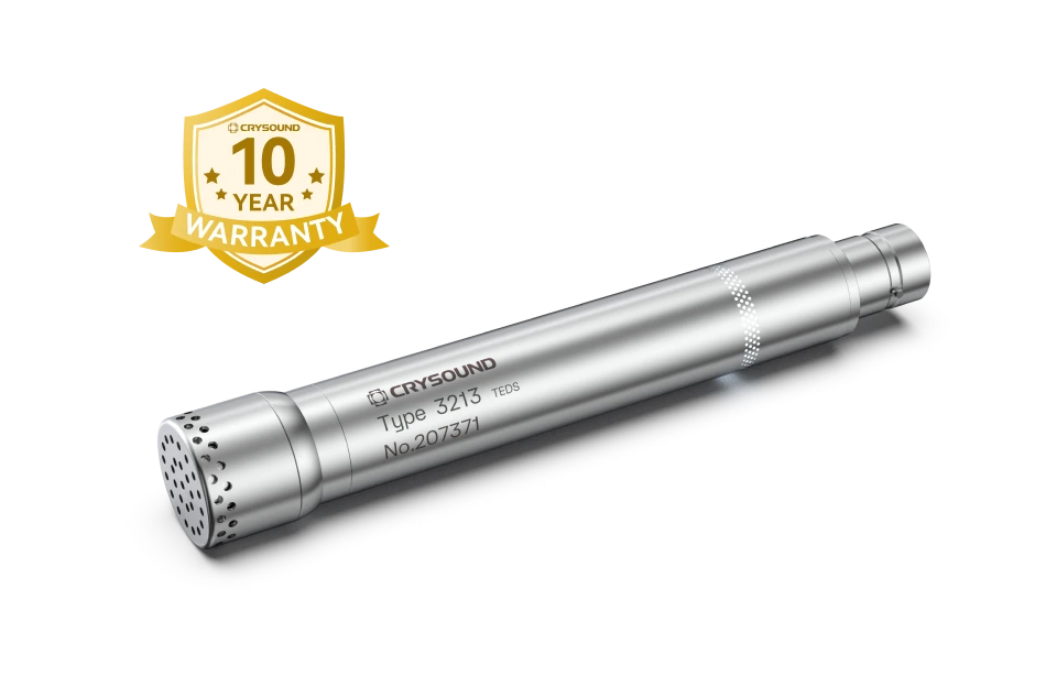
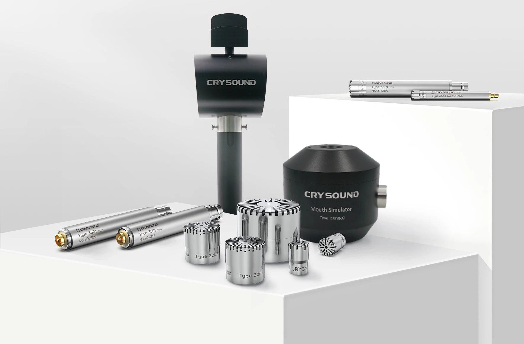
Products

Featured Products

Product Lines

Deliver reliable products for acoustic measurement and testing

Sensors

Provides measurement microphones, mouth simulators, ear simulators, and more for accurate acoustic measurements.
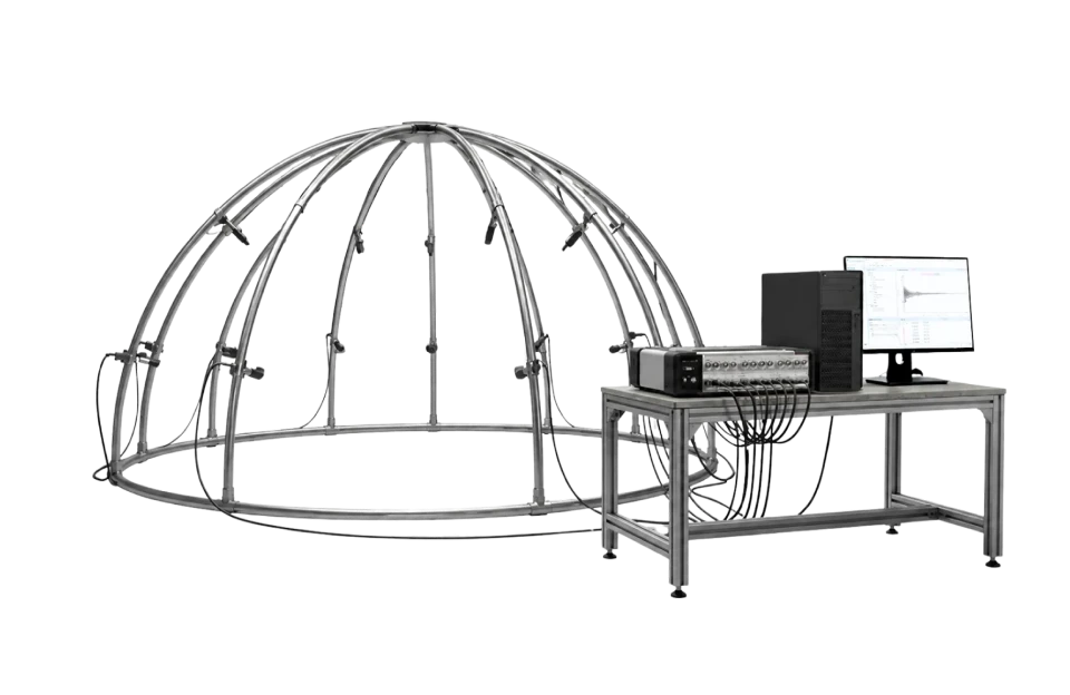
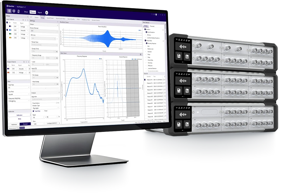
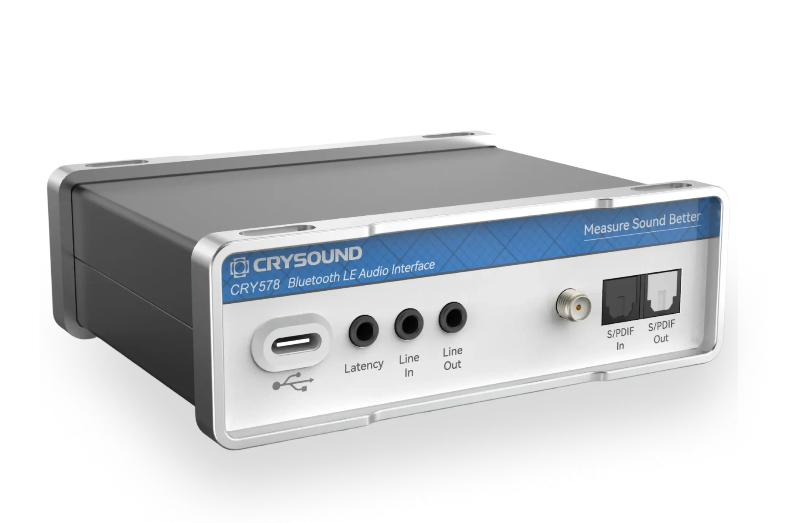
Data Acquisition

Combines hardware and software for high-speed, high-precision signal acquisition, ideal for various acoustic applications.
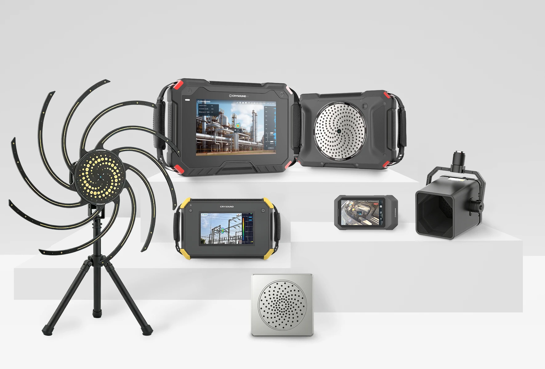
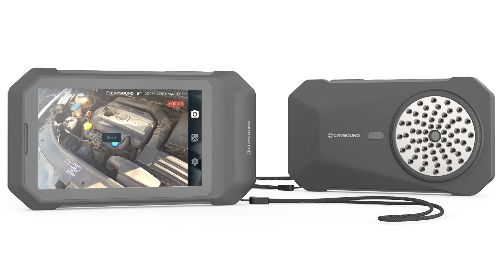
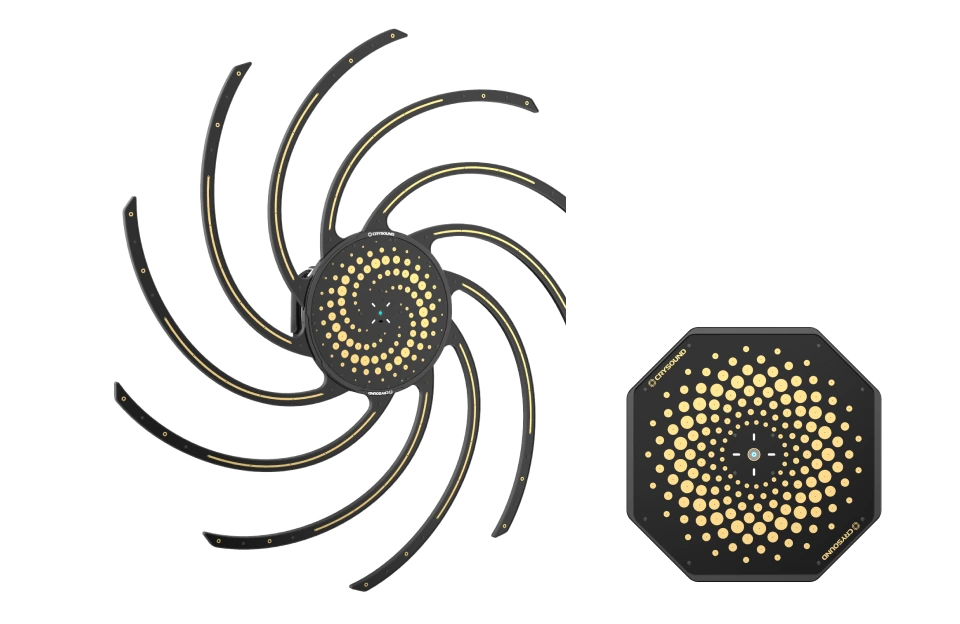
Acoustic Imaging

Offers acoustic cameras for gas leak detection, partial discharge, and fault diagnostics across handheld, fixed, and UAV platforms.
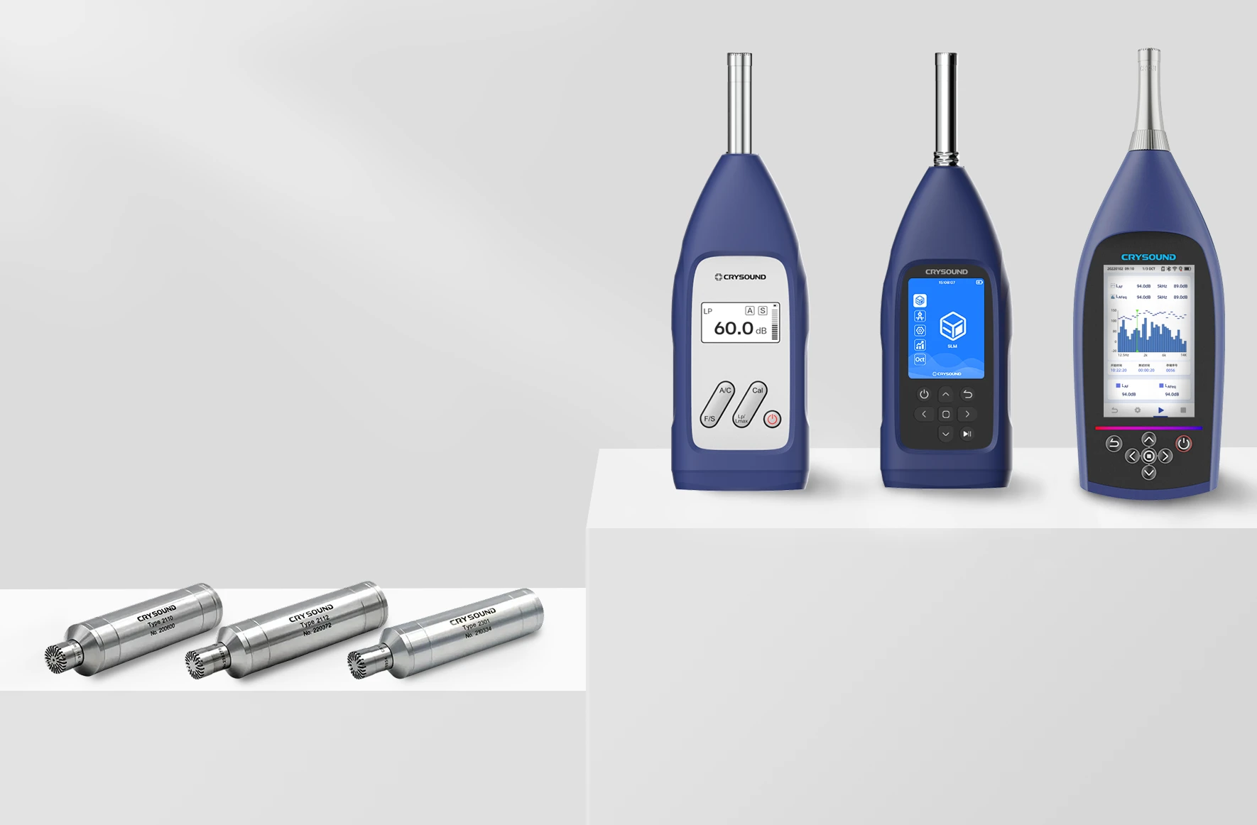
Noise Measurement

Includes sound level meters, noise sensors, and monitoring systems for effective noise measurement and analysis.

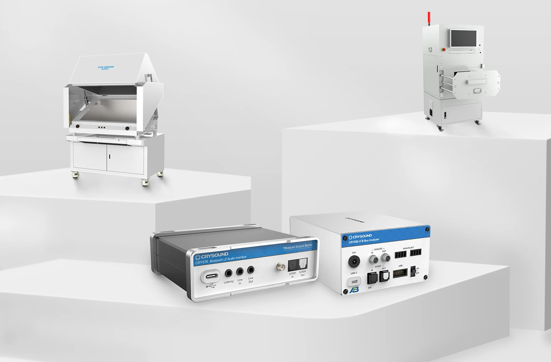
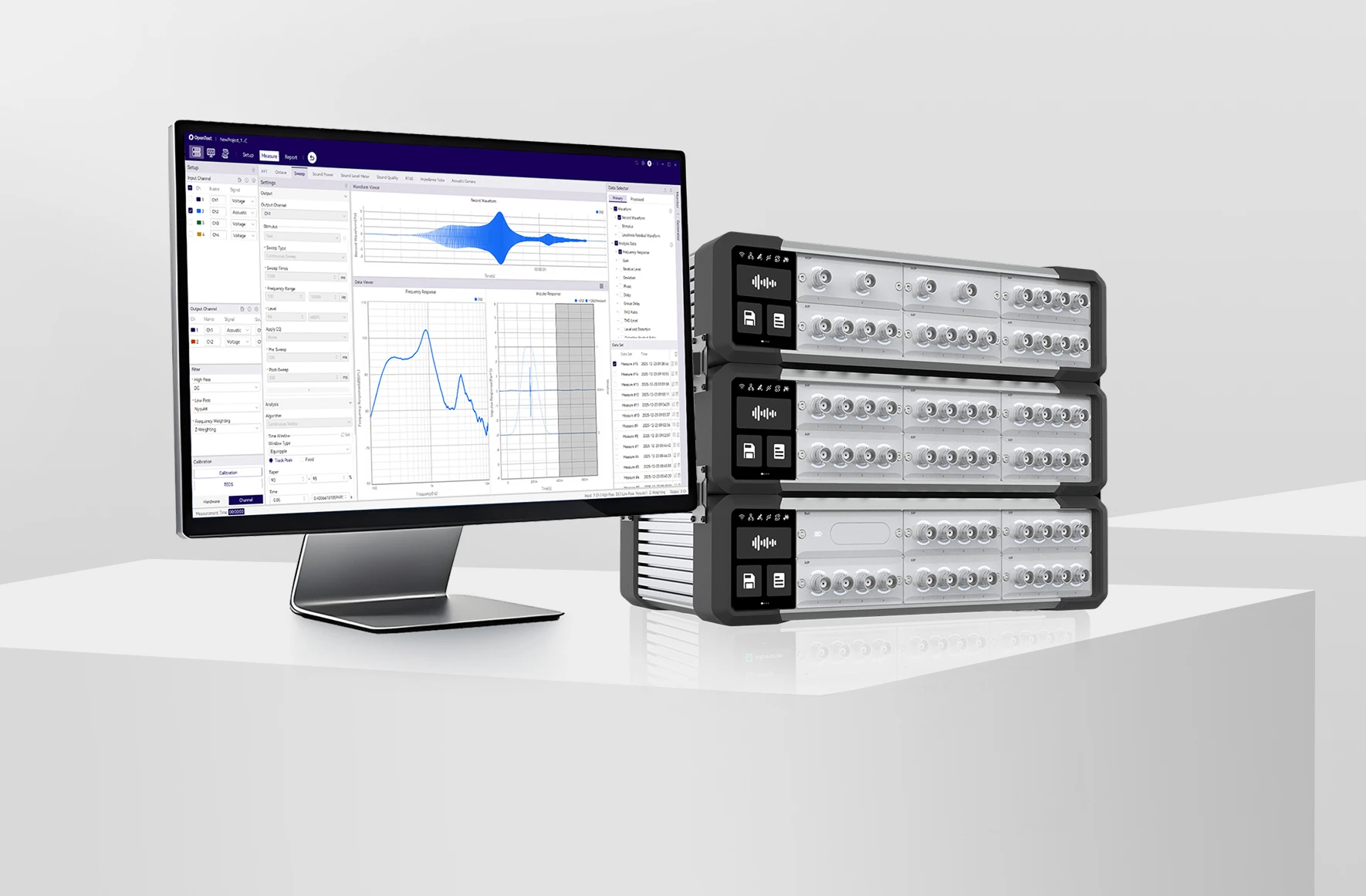
Electroacoustic Test

Delivers complete electroacoustic testing solutions, including analyzers, testing software, and acoustic test boxes.

Solutions

Provide high-quality solutions for the acoustic field

Monitor all industrial noise and regulate pollution properly, fostering industrial-community harmony.
CRYSOUND provides a shell-type dual-box four-measurement solution for headphone ANC&ENC testing.
In recent years, AR/VR (Augmented Reality/Virtual Reality) technology has
Acoustic imaging technology provides an ultrasonic method for composite airtightness inspection—faster and more reliable.

Blogs

Share insights, cases and trends in acoustic testing

CRYSOUND 10-Year Warranty for CRY3000 Series Sensors

Precision measurement is only as trustworthy as the tools behind it. At CRYSOUND, long-term reliability has always been part of how we support professional acoustic testing and metrology work—especially for equipment expected to perform consistently over many years. That's why CRYSOUND provides a 10-Year Limited Warranty for eligibleCRY3000 series sensors offering long-horizon confidence for labs, manufacturers, and audio professionals who depend on stable performance. What the 10-year warranty covers This is a limited warranty focused on defects in materials or workmanship that occur under normal use, installation, and maintenance conditions. It is not a guarantee of fitness for a specific purpose. Eligible product categories (CRY3000 Series) The 10-year limited warranty applies to the following CRY3000 Series categories (traceable by product nameplate/serial number):Microphones Preamplifiers Microphone Sets Mouth Simulators Ear Simulators Ear Simulator Sets. Warranty term: 10 years (and what's different) For the main product categories above, the warranty term is 10 years.Accessories/consumables (e.g., windscreens, cables, adapters, seals, replaceable pinnae, packaging) are covered under a 6-month warranty unless otherwise specified by contract or separate terms. When the warranty period starts The warranty period is calculated from the shipping/delivery date. If that date is unavailable, it is calculated from the end-user purchase date (with contract proof). If valid proof cannot be provided, CRYSOUND may use the factory date or the latest traceable serial-number record as the basis. What CRYSOUND will do for eligible defects If CRYSOUND confirms the issue is covered, we may provide one or more of the following: Free repair, including necessary parts and labor Replacement with the same model, or a model of equal or higher performance (new or certified refurbished/remanufactured) Customized/project products follow contract terms Repairs or replacements do not extend the original warranty period. Clear boundaries (typical exclusions) As a limited warranty, it excludes issues caused by misuse, drops/crushing, liquid ingress, corrosive environments, out-of-spec power/ESD/surge, improper installation/grounding/sealing/maintenance, unauthorized disassembly/modification, missing/altered serial numbers, normal wear/cosmetic changes, shipping/storage mishandling, or third-party compatibility problems (where applicable). Calibration note (important for metrology users) Because microphones and simulators are metrology instruments, slight drift can occur due to environment and measurement uncertainty. Unless drift is confirmed to be caused by a manufacturing defect, calibration/recalibration and certificate updates are typically not included for free (paid calibration/verification services may be available). Service logistics (shipping & service location) For in-warranty cases, users typically cover round-trip shipping to CRYSOUND/authorized service points. Cross-border service may involve duties or customs clearance fees unless otherwise agreed by contract. CRYSOUND will arrange the nearest service option based on region, product type, and spare-part availability. Warranty & Support To request warranty service or technical support, contact info@crysound.com (or reach out to your CRYSOUND sales contact). See the warranty policy on our website: https://www.crysound.com/warranty/

What Does “1000 V Isolation” Actually Isolate?

In many practical applications, data acquisition is not performed in an “ideal laboratory” environment. The device under test may be connected to mains power, distribution cabinets, frequency converters, or large electromechanical systems, while the acquisition card on the other side is connected via USB or Ethernet to a computer—sometimes operated directly by a person. These two sides are often not at the same electrical potential. If there is no effective electrical isolation inside the data acquisition card, this potential difference may propagate through signal lines, shields, or ground paths to the system side, leading to measurement distortion, interface malfunction, or even safety hazards. This is the fundamental reason why isolation exists in data acquisition systems. What Is the Isolation Rating of a Data Acquisition Card? In a data acquisition system, the isolation rating is not a simple voltage number, nor is it equivalent to “the voltage that the input can directly withstand.” It describes whether there is a reliable electrical isolation barrier between the measurement side (connected to sensors and the device under test) and the system side (connected to the host computer, communication interfaces, and power supply), and under what level of voltage stress this isolation remains valid. Isolation principle You can think of isolation as a bridge between two islands: The bridge allows information to pass—measurement data, digital communication, control signals. But it blocks dangerous currents—fault currents, ground-loop currents, and energy that could carry high potential to the host side. For this reason, isolation in data acquisition systems typically addresses both safety and measurement stability at the same time. Why Is Isolation Often More Important Than Accuracy Specifications? In many field applications, engineers do not encounter problems such as “insufficient resolution,” but instead: The same system works well in the lab, but noise increases dramatically on site. Once multiple devices are connected together, the data begins to drift. Replacing the computer or using a different power outlet suddenly makes the problem disappear. The common root cause behind these phenomena is often not algorithms or ADC performance, but rather improper handling of electrical potential relationships within the acquisition system. The value of isolation lies precisely here: by breaking unnecessary current loops and limiting the propagation paths of common-mode voltage and fault energy, isolation allows the acquisition system to behave in a controlled and predictable manner even in complex electrical environments. In industry discussions, the core values of isolation usually fall into three categories: signal integrity, safety, and instrument protection. Signal Integrity: Breaking Ground Loops and Improving Common-Mode Rejection Many cases of “inaccurate measurement” are not caused by ADC resolution, but by unwanted currents flowing through ground wires or shields. When the device under test and the host computer, enclosure, or other equipment are at different ground potentials, connecting them via signal cables may form ground loops. Power-line interference and electromagnetic noise then appear as “baseline noise” or ripple in the waveform. Isolation improves this by breaking the current loop paths. Safety: Confine High Potential and Fault Energy to the Measurement Side When measurement points are located near mains power, distribution cabinets, or frequency converters, the real risk is not merely “high voltage,” but where abnormal voltage or fault energy may propagate. If there is no clear electrical isolation between the measurement side and the host side, this energy may travel through signal or ground connections into the computer or communication interfaces, causing equipment damage or safety hazards. Isolation establishes a clear internal safety boundary: high potential and uncertain electrical environments are confined to the measurement side, while the system side—where the host computer and operator reside—remains within a controlled and safe potential range. If an abnormal condition occurs, the problem is contained on the measurement side and does not propagate further. Instrument Protection: A Larger Measurable Window Under High Common-Mode Voltage A non-isolated acquisition system effectively binds the measurement reference ground to system ground or earth. As a result, the measurable input range is centered around earth potential. If the entire signal shifts to a high common-mode potential, the front-end amplifier or ADC may exceed its allowable range or even be damaged. An isolated system allows the measurement reference to “float,” enabling the input measurement window to be centered around the isolated local ground. This permits operation under much higher common-mode voltages, with the ultimate limits determined by the isolation barrier and input protection circuitry together. Commonly Confused Isolation-Related Terms Isolation is often misunderstood because a single term—“isolation voltage”—is used to answer very different questions. The following clarifies these related but distinct concepts. Common-Mode Voltage Common-mode voltage refers to the voltage that is simultaneously applied to both measurement inputs relative to the acquisition system reference ground. It is not the signal of interest. The measurement signal concerns the difference between two input terminals, whereas common-mode voltage describes how high the two terminals are elevated together relative to ground. For example, in battery stacks or floating power systems, the signal itself may be only a few volts, but the entire source may be elevated tens or hundreds of volts above the acquisition card ground. In industrial environments, ground noise or electromagnetic interference may also impose time-varying AC voltage on both measurement leads. These “collectively elevated or oscillating voltages” constitute common-mode voltage. Working Voltage Working voltage is the voltage that can be continuously applied to a device over long periods. It is typically understood as the combination of measured voltage and common-mode voltage, and represents the condition under which the device can operate reliably over time. Withstand Voltage Withstand voltage refers to whether the isolation barrier can survive a very high voltage applied for a short duration without breakdown or damage. To verify this, a dielectric withstand (hipot) test is typically performed. During such a test, a voltage significantly higher than normal operating conditions is applied across the isolation barrier for approximately one minute. If no breakdown, abnormal leakage, or functional damage occurs, the isolation barrier is considered electrically robust. It is critical to note that withstand voltage does not indicate that the device can operate continuously at that voltage. It is a safety and quality verification metric, demonstrating that the insulation will not fail immediately under abnormal or extreme conditions. Input Overvoltage Protection Input overvoltage protection specifies the maximum allowable differential voltage between the positive and negative terminals of the same input channel. Exceeding this limit may damage the input circuitry. This is fundamentally different from isolation withstand voltage: Isolation withstand voltage applies between the measurement side and the system side. Overvoltage protection applies between the positive and negative terminals of the same channel. Measurement Category (CAT) Measurement category defines the severity of transient overvoltage that a measurement system may encounter in its electrical environment. Categories increase from CAT I to CAT IV: CAT I: Low-energy electronic circuits. CAT II: Household appliances and receptacle outlets, typically protected by indoor distribution panels. CAT III: Industrial distribution cabinets and environments with large motors, pumps, or compressors, subject to switching transients and inductive load surges. CAT IV: Outdoor power distribution points exposed to surges and lightning strikes. Pollution Degree Pollution degree describes environmental factors such as dust, moisture, and condensation that affect insulation surfaces. Higher pollution degrees reduce effective insulation performance, requiring higher baseline insulation strength. What Does "1000 V Isolation" Actually Mean? When a specification states “1000 V isolation,” three immediate questions must be asked, otherwise the number has no real comparability: Is it AC or DC? Is it Vrms, Vpk, or Vdc? Is it withstand voltage (short-term) or working voltage (long-term)? What exactly is isolated? Channel-to-ground? Channel-to-channel? Measurement side to USB/host side? The most important takeaway is this: “1000 V isolation withstand” does not automatically mean the system can continuously operate at 1000 V common-mode voltage, nor does it mean that 1000 V can be directly applied to the input. Continuous capability depends on working voltage, measurement category, input overvoltage protection, and the entire system chain including sensors, cables, and terminals. How Isolation Is Implemented: Isolation Barriers and Signal Transfer Methods Isolation is not simply “air separation,” but a combination of structure, materials, and signal-coupling mechanisms. Common isolation signal-transfer methods include: Inductive / Transformer-Based Isolation Inductive isolation transmits energy or information via magnetic fields rather than direct electrical conduction, fundamentally based on Faraday's law of electromagnetic induction. Inductive isolation chip block Inside the chip, planar coils are fabricated on silicon or within the package, forming transformer-like structures. Transmitter side: current → coil → alternating magnetic field Receiver side: magnetic field variation → induced voltage → signal recovery Advantages include very high common-mode transient immunity (CMTI), high speed, low jitter, long-term stability, and excellent channel consistency. Disadvantages include higher power consumption and cost compared with capacitive isolation. Capacitive Coupling Capacitive isolation uses the “DC-blocking, AC-passing” property of capacitors to achieve voltage isolation, relying on electric-field variation within the dielectric. Capacitive isolation chip block Signal variation → electric-field variation → displacement current coupling Advantages include low power consumption, small die area, high integration, lower cost, and high speed. Disadvantages include higher sensitivity to common-mode dv/dt, stricter PCB symmetry requirements, and higher dependence on reference-ground layout. Optical Isolation Optical isolation uses light as the isolation medium, with air or transparent insulation providing physical separation. The principle is photoelectric conversion plus spatial isolation. Optical isolation chip block Electrical signal → LED emission → photosensitive device → electrical signal Advantages include simple structure, extremely high withstand voltage, good performance for low-frequency and switching signals, and strong EMC characteristics. Disadvantages include slower speed due to device latency, higher variability, and unsuitability for high-precision synchronous systems. Comparison of Isolation Technologies ItemInductiveCapacitiveOpticalWithstand voltage★★★★☆★★★☆★★★★★Transmission speed★★★★☆★★★★★★★Common-mode immunity★★★★★★★★☆★★EMI immunity★★★☆★★★★★★★★★Stability★★★★★★★★★★★Low power★★★★★★★★★★Suitable for DAQRecommendedRecommendedNot recommended A frequently overlooked but critical metric here is CMTI. In high dv/dt environments such as inverters, SiC/GaN power supplies, and motor drives, the issue is often not how high the static common-mode voltage is, but how fast it changes. Rapid high-voltage transients may couple through parasitic capacitances across the isolation barrier, disrupting or corrupting data transmission. Therefore, isolation must withstand not only voltage magnitude, but also voltage transition speed. Common Isolation Topologies in Data Acquisition Before asking whether a DAQ card is isolated, a more important question should be asked: where is the isolation applied? Different products may use entirely different isolation domains, resulting in very different capability boundaries and application suitability. Common DAQ isolation topologies include: Channel-to-system-ground isolation Bank (group) isolation Channel-to-channel isolation Channel-to-System-Ground Isolation Definition: Each channel (or group of analog front ends) is isolated from system ground and host ground, while channels typically share a common reference ground. Channel-to-system-ground This topology can: Break ground loops between the measurement side and the host side. Prevent high potential or fault energy from reaching the computer, USB, or network interface. Significantly improve stability when measurement and host grounds differ. The entire DAQ effectively “floats” with the device under test, while the host remains on the safe side. Suitable scenarios include industrial field measurements where all channels share the same potential. Bank Isolation Definition: Channels are divided into groups (banks). Each bank has its own isolation domain, with isolation between banks and between each bank and system ground. Bank isolation This topology allows multiple independent systems to be measured simultaneously while preserving multi-channel synchronization within each bank, balancing cost, size, and isolation capability. Channel-to-Channel Isolation Definition: Each channel has a fully independent isolation domain and reference ground. Channel-to-channel isolation Each channel effectively functions as an independent isolated acquisition system, suitable for battery stacks, distributed measurements, and scenarios with large inter-channel potential differences, at the expense of higher cost, size, and system complexity. Isolation Selection: From Parameters to Practical Judgment After understanding isolation concepts, topologies, and voltage ratings, the key question becomes: does a given isolation design truly fit the application? Many misjudgments arise from focusing on a single number such as “1000 V isolation” without clarifying where isolation is applied, for how long, and what additional protections are required. What Is Being Isolated, and Where Does the Isolation Occur? If all measurement objects belong to the same system and there is no potential difference between them, a Channel-to-System Ground Isolation data acquisition card should be selected. If the measurement objects belong to multiple different systems, but the measurement points within each system share the same ground reference, a Bank Isolation (group isolation) architecture should be selected. In this case, measurement points from different systems must not be connected to the same bank of the acquisition card. If all measurement objects belong to the same system but there are significant potential differences between them, a Channel-to-Channel Isolation data acquisition card should be selected. This is the prerequisite for evaluating all isolation-related parameters.If the isolation location is unclear, other voltage specifications are almost meaningless for comparison. Isolation Withstand Voltage of a Data Acquisition System At a minimum, the following information must be clearly specified:whether the voltage is AC or DC, the duration (typically a 1-minute withstand test), and only then the voltage value itself. If a data acquisition card specifies an AC isolation voltage of 1000 V, it means that an AC voltage with a peak value of ±1414 V is applied between the circuit grounds on both sides of the isolation barrier, and after 1 minute the leakage current remains below 0.1 mA. If a data acquisition card specifies a DC isolation voltage of 1000 V, it means that a +1000 V or −1000 V DC voltage is applied between the circuit grounds on both sides of the isolation barrier, and after 1 minute the leakage current remains below 0.1 mA.However, one must not assume that ±1000 V AC can be applied in this case—the two are not equivalent, because different devices have different withstand capabilities for AC and DC voltages. It should be emphasized that the withstand voltages discussed above are short-term withstand ratings. They do not mean that the device can operate continuously at a 1000 V common-mode voltage. They only indicate that the device will not be damaged under those conditions, not that normal operation is guaranteed. Maximum Common-Mode Operating Voltage This is the parameter that deserves particular attention when selecting a data acquisition card. In most cases, it refers to the long-term voltage difference between the measurement side and the system ground. For example, if we want to measure the current on a 220 V mains line, the corresponding common-mode voltage is: 220 V × 1.414 = 311 V Allowing at least a 50% margin, the data acquisition card should therefore support a maximum common-mode operating voltage greater than 466 V. If a specification sheet only provides isolation withstand voltage but does not clearly specify working voltage or maximum common-mode range, extreme caution is required in practical use. Input Voltage Range The input voltage range is also referred to as differential voltage. It defines how much voltage difference the input terminals of a channel can tolerate. The key question is what happens when this limit is exceeded:is the signal clipped, is the input shut down, or is permanent damage caused? This parameter determines whether the device can protect itself under wiring errors or abnormal conditions, or whether it will fail catastrophically. If the distinction between common-mode voltage and differential voltage is still unclear at this point, the following analogy may help. Measuring Across a River In the diagram, the person cannot approach the apple directly because of the river acting as an isolation barrier, so a caliper with an extended handle is used to measure the apple on the opposite bank. The 300 cm distance across the river corresponds to the common-mode voltage in the system, while the measurement range of the caliper (20 cm) corresponds to the differential voltage range. Isolation Structure of the SonoDAQ Module (Bank Isolation Example) After distinguishing between channel-to-ground isolation, bank isolation, and channel-to-channel isolation, as well as various isolation parameters, the next question for a specific product is: where exactly is the isolation boundary drawn? The following figure shows the isolation structure of a SonoDAQ module, illustrating the division of its isolation domains. SonoDAQ Module Isolation From the module structure, it can be clearly seen that SonoDAQ Pro adopts a bank isolation architecture (see Section 6.2). Each module is isolated from the host, while the four channels on each module are not isolated from each other. The module divides functionality and electrical domains into three parts: Measurement Side: Located on the left side of the module, directly connected to sensors and the device under test. This belongs to the measurement-side electrical domain and may be at a high or uncertain common-mode potential. Bank Isolation Domain: Located in the middle of the module, this is the primary isolation barrier between the measurement side and the system side. Multiple channels within the same bank share a common measurement-side reference ground and are collectively isolated from the system side through this isolation domain. As shown in the diagram, two types of isolation circuits are used: capacitive isolation for digital communication and magnetic (transformer-based) isolation for power. System Side: Located on the right side of the module, communicating with the host through the backplane. This side operates under system ground reference and connects to processors, communication interfaces, and the host computer. From Concept to Verification: Isolation Must Be Proven, Not Assumed Through the previous discussion, we have distinguished between differential and common-mode voltages and understood the respective roles of isolation withstand voltage, working voltage, and common-mode capability. While these concepts are not complex in specifications or standards, a more critical question remains in real engineering practice: Do these isolation boundaries actually hold under real-world conditions as the parameters suggest? For example, when the device under test operates at a high common-mode potential, the acquisition system must run online for extended periods, and the host computer and operators must always remain on the safe side. Simply “trusting a specification value” is far from sufficient. Rather than staying at the conceptual level, it is better to return to engineering practice. The following two experiments are not intended to demonstrate extreme parameter limits, but to address a more practical question. For this purpose, SonoDAQ Pro was selected as the test platform—not because of exceptionally high specifications, but because its isolation structure is clear and its boundaries are well defined, making it suitable for engineering-level isolation verification. The experiments are conducted from two perspectives: withstand voltage testing (hipot) and mains-powered incandescent lamp current measurement. Withstand Voltage Test (Hipot) Test objective: To verify that the isolation barrier can withstand high voltage under specified conditions without breakdown, providing an intuitive engineering verification result The general industry definition of dielectric withstand testing is to apply an elevated voltage across an insulation barrier for approximately 1 minute. Passing the test indicates that the insulation system has sufficient electrical strength under those conditions, while also clarifying the purpose and limitations of the test to avoid misinterpretation. Test equipment: WB2671 hipot tester Test conditions: 1000 V DC, duration 1 minute, leakage current threshold 0.1 mA Withstand Voltage Test Test Results 1.02 kV DC, duration 1 minute, leakage current = 0.03 mA, with no breakdown, flashover, or arcing observed. Explanation: SonoDAQ Pro adopts a bank isolation architecture, where the six slots are isolated from each other. Therefore, during testing, the hipot voltage was applied between Channel 1 of two adjacent modules. 220 V Mains Incandescent Lamp Current Measurement Experiment Test objective: To demonstrate how the data acquisition card can measure signals in a high-voltage system under real mains conditions, and to verify measurement correctness. Why an incandescent lamp? Its steady-state behavior closely resembles a resistive load, making current waveforms intuitive and easy to interpret. The cold filament has low resistance, producing a clear inrush current at power-on, which is suitable for demonstrating transient capture and trigger recording capability. 220 V Mains Incandescent Lamp Current Measurement Wiring In the diagram, the left side is the high-voltage area directly connected to the 220 V AC source. After all wiring is completed, the power plug is inserted. The right side contains the isolated data acquisition card, forming the low-voltage area. The computer and operator remain entirely on the safe side. The experiment used SonoDAQ Pro hardware with OpenTest software. The incandescent lamp was rated at 220 V / 60 W. The following photos show the setup before power-on (left) and after power-on (right). 220 V Mains Incandescent Lamp Current Measurement Test configuration: sampling rate 192 kSa/s, AC coupling for the input signal. The acquisition card directly measured the voltage across a 1.4 Ω shunt resistor. Using the “Record” function in OpenTest, the entire power-on and power-off process was recorded. Steady-State Current Waveform Steady-state current:Vrms = 386 mV → Irms = 386 / 1.4 = 275.7 mAFrequency f = 49.962 Hz Startup Transient Current Startup current:Vpeak = 2.868 V → Ipeak = 2.868 / 1.4 = 2.05 A Crest factor calculation:CF = Ipeak / Irms = 2.05 / 0.2757 = 7.44 Incandescent lamp power calculation:P = 220 V × 0.2757 A = 60.65 W Conclusion SonoDAQ Pro can accurately measure the operating current of an incandescent lamp connected directly to the mains without using a current transformer. This experiment does not merely verify whether mains signals can be measured; it verifies whether isolation can simultaneously ensure system safety and measurement accuracy when the device under test operates at a high common-mode potential over extended periods. Isolation Is Not a Parameter, but a Boundary Isolation is not “a single voltage value,” but rather defines where risk is confined and whether signals can still pass reliably. A reliable isolation solution is the result of structure, parameters, topology, and application scenario all being valid at the same time. To see more imformation about the SonoDAQ, please fill in the form below, and we will recommend the best solution to address your needs.

What are Sound Pressure, Sound Intensity, and Sound Power?

Sound is everywhere in our daily life: birdsong, street noise, engine roar, even the faint airflow from an air conditioner. For people, sound is not only about whether we can hear it, but whether it feels comfortable, is disturbing, or poses a risk. The same 70 dB can feel completely different; and when something feels "noisy", the cause may come from the source itself, the propagation direction, or reflections from the environment. When we turn this "perception" into quantifiable engineering data, the three most easily confused concepts are sound pressure, sound intensity, and sound power. They answer: Sound pressure: how loud it is at a specific point; Sound intensity: how much sound energy is propagating in a particular direction; Sound power: how loud the source is in terms of its total acoustic emission; This article explains sound pressure, sound intensity, and sound power in an intuitive way, so you can better understand sound. Sound Waves In engineering acoustics, sound pressure, sound intensity, and sound power are three fundamental and important physical quantities. Before introducing them in detail, we need the concept of a sound wave. A vibrating source sets the surrounding air particles into vibration. The particles move away from their equilibrium position, drive adjacent particles, and those adjacent particles generate a restoring force that pushes the particles back toward equilibrium. This near-to-far propagation of particle motion through the medium is what we call a sound wave. Figure 1. Propagation of a Sound Wave in Air Sound Pressure When there is no sound wave in space, the atmospheric pressure is the static pressure p0. When a sound wave is present, a pressure fluctuation is superimposed on p0, producing a pressure fluctuation p1. Here p1 is the sound pressure (unit: Pa). Therefore, sound pressure is the instantaneous deviation of the air static pressure caused by the sound wave. The human brain does not respond to the instantaneous amplitude of sound pressure, but it does respond to the root-mean-square (RMS) value of a time-varying pressure. Therefore, the sound pressure p can be expressed as: In practical engineering applications, the sound pressure level Lp: where Pref = 2 × 10⁻⁵ Pa is the reference sound pressure. In practice, we usually use sound pressure level (dB) to characterize sound pressure, rather than using pressure in pascals. Why? Figure 2 answers this well. From a library to the entrance of a high-speed rail station, sound pressure may increase by a factor of 100, while sound pressure level increases by only 40 dB. This reflects the difference between a linear scale and a logarithmic scale. From an engineering perspective, using sound pressure directly leads to large numeric variations that are inconvenient for evaluation. Moreover, the human auditory system is closer to a logarithmic response, so sound pressure level better matches hearing. Figure 2. Sound Pressure and Sound Pressure Level Sound Intensity Sound intensity describes the transfer of acoustic energy. It is the acoustic power passing through a unit area per unit time. It is a vector quantity that is directional, with units of W/m2, defined as the time average of the product of sound pressure and particle velocity: where v(t) denotes the particle velocity vector. Under the ideal plane progressive-wave approximation, sound pressure and particle velocity approximately satisfy: where ρ is the air density, c is the speed of sound. Therefore, the magnitude of sound intensity along the propagation direction can be written as: Similarly, sound intensity has a corresponding intensity level LI: where I0 = 10-12 W/m2 is the reference sound intensity. Compared with sound pressure level measurements, sound intensity measurements have the following characteristics: Directional:it can distinguish whether acoustic energy is propagating outward or flowing back, so under typical field conditions it is often less sensitive to reflections and background noise; Source localization:intensity scanning can directly reveal the main radiation regions and leakage points, making remediation more targeted; Higher system complexity:it typically requires an intensity probe, with higher overall cost and more setup and calibration effort; Figure 3. Sound Intensity Testing A key advantage of sound intensity measurement in engineering applications is that it characterizes both the direction and magnitude of acoustic energy flow. It can separate the contributions of outward radiation from the source and reflected backflow from the environment, so under non-ideal field conditions it tends to be less affected by reflections and background noise. In addition, the sound intensity method can obtain sound power directly by spatially integrating the normal component of intensity over an enclosing surface. Combined with surface scanning, it can identify dominant source regions and locate leakage points. Therefore, it is highly practical and interpretable for noise diagnosis, verification of noise-control measures, and sound power evaluation. The key instrument for sound intensity testing is the sound intensity probe. Unlike a single microphone, an intensity probe is not used merely to measure “how large the pressure is”; it must provide the basic quantities required for calculating intensity (sound pressure and particle velocity). Therefore, the probe typically outputs two synchronous channels and, together with a two-channel data-acquisition front end and dedicated algorithms, yields intensity results. In engineering practice, the probe often includes interchangeable spacers, positioning fixtures, and windshields. Channel amplitude/phase matching, phase calibration capability, and airflow-interference mitigation directly determine the credibility and usable frequency range of intensity measurements. Two types of sound intensity probes are commonly used: P-U probes (pressure-particle-velocity) and P-P probes (pressure-pressure). A P-U probe consists of a microphone and a velocity sensor, measuring sound pressure p(t) and particle velocity v(t) simultaneously. The principle is more direct, but particle-velocity sensors are often more sensitive to airflow, contamination, and environmental conditions, requiring more protection and maintenance in the field and usually costing more. Figure 4. P-U Sound Intensity Probe (Microflown) A P-P probe uses two matched microphones aligned on the same axis. It uses the two pressure signals p1(t) and p2(t) to estimate the particle-velocity component v(t). However, it is sensitive to inter-channel phase matching and the choice of microphone spacing - the spacing determines the effective frequency range: a larger spacing benefits low frequencies, but high frequencies suffer from spatial sampling error; a smaller spacing benefits high frequencies, but low frequencies become more susceptible to phase mismatch and noise. Figure 5. P-P Sound Intensity Probe (GRAS) P-U probes are relatively niche, mainly because it is difficult to make them both stable and inexpensive, and they generally have poorer resistance to airflow. P-P probes, thanks to their good field robustness and the ability to adjust bandwidth flexibly via microphone spacing, are currently the mainstream choice in engineering applications. Sound Power Sound power W is the rate at which a source radiates acoustic energy, with units of watts (W). For any closed measurement surface S enclosing the source, the sound power equals the integral of the normal component of sound intensity over that surface: where n is the unit normal vector pointing outward from the measurement surface. Sound power level Lw is defined as: where W0 = 10-12 W is the reference sound power. Figure 6. Sound Power Measurement Sound power characterizes a source's inherent acoustic emission capability: the total acoustic energy it radiates per unit time. It has little to do with measurement distance or microphone position, and ideally does not depend on how "loud" it is at a particular point in a room. This is fundamentally different from sound pressure and sound intensity. To better understand sound pressure, sound intensity, and sound power, you can imagine noise as water flow. Sound pressure is like the "water pressure" you feel when you put your hand at a certain location (it changes with distance to the nozzle, direction, and the shape of the basin). Sound intensity is like the instantaneous "direction and rate of flow" (it has direction and can even be reflected by walls, creating backflow). Sound power is like "how much water the nozzle sprays per second" - it is a property of the nozzle itself. In measurement, it is obtained by integrating the outward normal flow over a surface surrounding the device. Figure 7. Analogy of Sound Pressure, Sound Intensity, and Sound Power In real projects, the algorithms for sound pressure, sound intensity, and sound power are relatively mature. The hardest part is acquiring the signals accurately and obtaining results quickly. In particular, tasks such as multi-channel microphone arrays, sound intensity, and sound power impose three hard requirements on the data-acquisition front end: low noise and wide dynamic range, strict synchronization and phase consistency, and stable on-site connections and power. SonoDAQ + OpenTest is positioned to provide a "front-end acquisition + synchronous analysis" foundation for engineering acoustics, allowing engineers to focus more on operating-condition control and data interpretation. It delivers the most value in the following types of projects: Sound intensity diagnostics: dual-channel synchronous sampling plus better amplitude/phase consistency management provide a more stable data basis for P-P intensity probes and intensity scanning. Microphone array systems: better aligned with engineering deployment needs in channel scalability, synchronization, and cabling, making it suitable for building expandable distributed test platforms. Sound power and standardized testing: helps engineers quickly lay out measurement points, covering multiple international sound power test standards. With guided configuration, one-click testing, and automatic report export, it saves substantial time and effort for engineers. Figure 8. SonoDAQ + OpenTest To see more clearly how SonoDAQ is connected and configured, typical application cases (such as equipment noise evaluation, sound source localization, and sound power testing), and commonly used BOM lists, please fill in the form below, and we will recommend the best solution to address your needs.

Detect Valve Leakage with Contact Ultrasound

Valves are the "core control components" of pipeline systems. They perform four key functions—opening/closing, regulating, isolating, and directing—enabling precise control of fluid flow. Once sealing integrity fails, minor cases can lead to process upsets and energy losses, while severe cases may result in fires or explosions, toxic exposure, or environmental pollution. We built a valve leak application around the three things customers care about most on site—fewer missed detections and false alarms, better localization, and more reliable leak-rate estimation—by distilling them into an executable, traceable standardized workflow and closing the loop in the application for end-to-end deployment. Common Causes of Valve Internal Leakage What leads to valve leakage? We summarize it into the following four main causes: Normal wear and tear: Frequent opening and closing gradually wears the sealing surfaces; long-term scouring and erosion from the flowing medium can also degrade the seal fit. Process medium factors: Sulfur compounds and similar components in the medium can cause electrochemical corrosion; residual construction contaminants—such as sand, grit, and particles—can accelerate wear and scratch the sealing surfaces, leading to poor sealing. Improper operation and maintenance: Using an on/off valve for throttling, lack of routine cleaning and preventive maintenance, inadequate servicing, or improper/unsafe operation can all damage sealing surfaces or prevent full closure. Installation and management issues: Outdoor storage exposed to rain, ingress of mud and sand, and sandblasting/field conditions introducing grit or debris into the valve cavity can contaminate and scratch sealing surfaces, ultimately causing internal leakage. Figure 1. Illustration of Valve Internal Leakage When a valve is closed but the sealing surfaces do not fully mate, the pressure differential drives the medium to pass through small gaps from the high-pressure side to the low-pressure side, forming high-velocity micro-jets and turbulent flow. This leakage typically results in several observable signs, including sound/ultrasound, vibration, abnormal pressure behavior, and temperature anomalies or frosting. Figure 2. Symptoms of Valve Leakage Why Contact Ultrasound Works When a valve seal fails, high-pressure fluid passing through tiny gaps at the sealing surfaces generates turbulent flow, producing high-frequency ultrasonic signals in the 20–100 kHz range. The signal intensity is generally positively correlated with the leak rate—the larger the leak, the higher the amplitude. In the field, you can capture ultrasonic signals at measurement points upstream of the valve, on the valve body, and downstream, then apply algorithms to extract and analyze signal features to detect and localize internal leakage. Compared with traditional methods, temperature-based approaches are easily affected by heat conduction and are difficult to quantify; pressure-hold tests are time-consuming and poor at pinpointing the leak location; and listening by ear is inefficient, prone to missed detections and false alarms, and heavily dependent on individual experience. That's exactly why we launched this application—turning an experience-driven task into a standardized, process-driven workflow, supported by acoustics and data analytics. Figure 3. CRY8124 Acoustic Imaging Camera with IA3104 Contact Ultrasound Sensor Workflow and Key Capabilities More standardized workflow: turning on-site operation into guided testing In the CRY8124 valve leak application, the software features a standardized and visualized workflow. Operators follow on-screen prompts to place the contact ultrasound sensor on each measurement point in sequence and simply tap "Test". The results are displayed on the interface, and the algorithm automatically determines whether internal leakage is present after the test. Figure 4. Valve Leakage Detection Feature Page At the same time, the software provides standardized inputs for key parameters such as valve ID, valve type, valve size, medium type, and the upstream/downstream pressure differential. This means test results are easier to align across the same unit, different shifts, and different operators—making retesting and trend management much more consistent. Figure 5. Valve Leakage Detection Feature Page Smarter: automatic diagnosis + leak-rate estimation Our valve leak detection capability focuses on two key improvements: By analyzing the dB level at each measurement point and the features of the ultrasonic signal, the system automatically determines the internal leakage result based on algorithmic data, reducing reliance on manual interpretation. Built-in AI algorithms estimate the leak rate from ultrasonic features at the measurement points, providing a quantitative reference to support valve maintenance decisions. This is the core logic behind our emphasis on a "higher detection rate": when judgments rely less on subjective experience, missed detections and false alarms become far more controllable—especially in complex sites with many valves and multiple parallel branches. Application Scenarios Across different industries, there is a common need for valve leak detection: Figure 6: Application Scenarios Field Case Study Case : A Coal-to-Chemicals Plant in Inner Mongolia (Fuel Gas / Coal Gas System) Below is a real field test case of valve leak at a coal-chemical plant. Any internal leakage in fuel gas or coal gas systems can compromise isolation. If leakage exists, the downstream side may remain gas-charged, and the work area may still be exposed to risks of CO and sulfur-containing acid gases entering the zone—potentially leading to poisoning, fire, or even explosion hazards. Using contact ultrasonics, we performed on-site testing on the suspected valves, quickly identified the leakage points, and estimated the leak rate. This helped the customer turn "isolation confirmed" from an experience-based judgment into data-backed verification, prioritize corrective actions, reduce work risks caused by misjudged isolation, and ensure safer maintenance and stable operation. Figure 7. On-site Test Photos Valve type: Fuel gas compressor room bypass valve (butterfly valve). Test result: 19.8 L/min. Medium / pressure: Fuel gas (H₂, CO, CH₄), 3 MPa. Figure 8. Test Results Valve type: Fuel gas compressor room plug valve Test result: 1.7 L/min. Medium / pressure: Coal gas (mainly CO), 2.5 MPa. Figure 9. Test Results On-Site Test Method: Repeatable 5-Point Measurements Confirm Operating Conditions Ensure there is a pressure differential, and isolate interfering branches as much as possible. Key steps Close the valve to be tested. Open the upstream and downstream valves of the test section. Confirm a pressure differential between upstream and downstream gauges, and verify ΔP > 0.1 MPa. As shown in the figure below When testing Valve A for valve leakage: open Valves B and C, and close Valves A and D. When testing Valve B for valve leakage: open Valves A and C, and close Valves B and D. Figure 10. Valve Status Place Measurement Points (MP1–MP5) Cover upstream → valve core → downstream. MP3: Located at the valve core. MP2: Located 1–2 pipe diameters (D) upstream of the valve (place the point on the pipe wall away from the valve). MP1: Located upstream of the valve, 2–3D away from MP2. If space is limited, MP1–MP2 spacing can be shortened to 0.5D. MP4: Located 1D downstream of the valve (place the point on the pipe wall away from the valve). MP5: Located downstream of the valve, 1–2D away from MP4 (recommended on the pipe wall just after the valve flange). If space is limited, MP5–MP4 spacing can be shortened to 0.5D. D = pipe diameter Figure 11. Test Point Layout NoteFor small, flangeless threaded valves, the spacing between measurement points should be at least three pipe diameters (3D). Fugure12. Test Point Layout FAQ We've listed some common scenario-based questions about valve internal leakage to help you understand the application faster and choose the right solution more efficiently. Q1. How do I choose a Contact Ultrasound Sensor for pipelines at different temperatures? A1. We recommend the following sensor selection based on pipe surface temperature: For low-temperature pipes (below -20°C) or high-temperature pipes (above 50°C), use a needle-type Contact Ultrasound Sensor. For temperatures between -20°C and 50°C, use a ceramic Contact Ultrasound Sensor for signal capture. Q2. Which valves can be tested for valve leakage? A2. This method is suitable for valve leakage detection across a wide range of valve types, including: Gate valves Plug valves Globe valves Ball valves Check valves Butterfly valves Needle valves Pressure relief valves Pinch valves If your valve type is not listed above, please feel free to contact us. Q3. Can we still test if the valve and pipe are insulated? A3. If the insulation fully covers the valve and pipeline, testing may not be possible. You'll need to remove the insulation at the measurement area, or leave an opening of about 7 cm in diameter so the Contact Ultrasound Sensor can directly contact the pipe wall to capture the signal. Q4. What should we pay attention to regarding the pipe surface during data collection? A4. The Contact Ultrasound Sensor must make good contact with a solid surface to reliably capture ultrasonic signals propagating through the pipe. Large particles or debris between the sensor and the pipe surface can lead to inaccurate results. If the pipe wall is rusty, wipe off any large dust or loose particles on the surface before testing. Contact Us If you'd like to learn more about how CRYSOUND acoustics can be applied to valve leak detection, or if you want a more suitable inspection solution based on your on-site process conditions and acceptance criteria, please contact us via the form below. Our engineers will get in touch with you.
Support Support
Product Catalogs Product Catalogs Solutions Solutions User Manuals User Manuals Software Download Software Download Product Inquiry Product Inquiry Schedule Demo Schedule Demo Technical Support Technical Support +86-571-88225128 +86-571-88225128
Request Quote 0
Request Quote