CRYSOUND POCKET Acoustic Imaging Camera Now Available on Kickstarter.
Blogs
In this article, we use a wind turbine blade factory as an example to show how CRY8124 Acoustic Imaging Camera can help complete a vacuum (negative-pressure) integrity test for a single blade in about 10 minutes. What Is a Wind Turbine Blade? Wind turbine blades are the key rotor components that convert wind energy into mechanical power, which is then turned into electricity by the generator. They are typically made of glass-fiber or carbon-fiber composite materials and offer a high strength-to-weight ratio and strong corrosion resistance. The wind turbines you see on mountain ridges, in deserts, or along coastlines rely on these large blades to capture energy efficiently. Why Vacuum Bag Integrity Testing Matters in Vacuum Infusion In wind turbine blade manufacturing, vacuum bag airtightness during the vacuum infusion process is critical for stable vacuum levels and consistent laminate quality. Even small leaks can lead to process instability, additional troubleshooting time, and rework risk. A typical workflow looks like this: 1. Preparation: Lay auxiliary materials (release fabric, flow media), seal the blade with vacuum film, block openings with sealing tape, and connect the vacuum pump, lines, and a gauge. 2. Evacuate to target vacuum: Start the pump and ramp to the process-defined vacuum level. If the target cannot be reached or keeps drifting, check high-risk areas first (especially sealant joints). 3. Vacuum hold & leak check: After reaching the specified vacuum level, turn off the pump and begin the hold phase (typically 10–30 minutes). Confirm the vacuum loss stays within your acceptance limit. If there is a leak, the vacuum level will drop noticeably—locate the leak point and repair it promptly. 4. Repair, re-test, document: Mark the leak points, replace any damaged vacuum film, and reseal the leaking areas. After repair, repeat evacuation and the vacuum hold test until the system meets the acceptance criteria, then document the results before proceeding to the next step. Common Challenges in Wind Turbine Blade Vacuum Bag Testing A single blade can be 60–100 m long, creating a large sealing perimeter—so leak hunting can push the test beyond 30 minutes. Dense laminate around the blade root makes leaks harder to locate with traditional methods. Manual checks are slow and operator-dependent, leading to inconsistent results across shifts. Case Study: Faster Leak Localization and Lower Rework Cost At one blade manufacturer, routine vacuum-hold tests after bagging sometimes failed the hold criteria, leading to repeated troubleshooting and rework. The team introduced the CRY8124 Acoustic Imaging Camera as an assistive tool to locate leaks faster during pre-infusion checks. Recommended Settings (Example) Turn on the CRY8124 and select the vacuum/leak scenario. Set the acoustic imaging band to 20–40 kHz. Adjust the imaging threshold (-40 dB to 120 dB) based on on-site conditions to reduce background noise from fans, cutting machines, and vacuum pumps. If ambient noise is high, enable focus/beamforming mode to further suppress environmental noise. On-Site Leak Scanning Workflow During inspection, the operator walks along key areas—such as the pressure side (PS), suction side (SS), the main-spar region, and around the root preform—while holding the CRY8124 Acoustic Imaging Camera. When a leak is present, the device overlays an acoustic “cloud map” on the live video feed, helping pinpoint the leak location and reducing repeated manual checks. Measured Impact (Customer-Reported) After introducing the CRY8124 Acoustic Imaging Camera, the average vacuum bag check time per blade dropped from 30+ minutes to around 10 minutes (about a 70% reduction in check time). The customer also reported annual cost savings exceeding $10,000 by reducing rework and scrap. How a 10-Minute Vacuum Bag Check Is Achieved The CRY8124 Acoustic Imaging Camera is designed for fast scanning across common blade inspection zones (PS/SS surfaces, main spar region, and the blade root). It provides a visual indication of leak location and relative leak severity, while using frequency filtering and beamforming to work in noisy production environments. With a high-density microphone array (up to 200 microphones, depending on configuration) covering 2 kHz–100 kHz, the system can capture ultrasonic components from small leaks and render them as an intuitive acoustic image. If you’d like to learn more about acoustic imaging for vacuum leak detection—or discuss your blade process and inspection targets—please use the “Get in touch” form below. Our team can share recommended settings and an on-site workflow tailored to your production conditions.
In acoustic design and noise control, a material’s acoustic impedance characteristics are a key factor in determining “how it sounds.” By measuring parameters such as the absorption coefficient, reflection coefficient, specific acoustic impedance, and acoustic admittance, we can not only quantify a material’s ability to absorb and reflect sound, but also evaluate its performance in real-world applications—such as room reverberation time, noise-control effectiveness in equipment, and the acoustic comfort of products like automobiles and home appliances. Accurate acoustic impedance testing gives engineers solid evidence for material selection, structural optimization, and acoustic simulation, dramatically reducing trial-and-error costs and shifting acoustic design from experience-driven to data-driven. Advantages of the Transfer-Function Method Among the many acoustic impedance measurement methods, the transfer-function method is widely used thanks to its fast testing speed, high accuracy, and broad applicable frequency range. By placing two microphones inside an impedance tube and using the sound-pressure transfer function, one can back-calculate parameters such as the absorption coefficient, reflection coefficient, and specific acoustic impedance—without complicated sound-source calibration or overly idealized assumptions about the sound field. Compared with the traditional standing-wave ratio method, the transfer-function method depends less on operator experience, delivers more stable low-frequency measurements, and is easier to automate and post-process, making it well suited for R&D, material screening, and high-throughput quality inspection in industry. CRYSOUND Integrated Test Solution CRYSOUND provides a complete acoustic impedance testing solution. Built around the CRY6151B data acquisition unit, and combined with our in-house algorithms plus testing software and an impedance-tube hardware system, it delivers an integrated workflow—from equipment calibration and data acquisition to parameter calculation and report generation. In terms of hardware configuration, we use a measurement chain optimized specifically for acoustic impedance testing. At the front end, two 1/4-inch pressure-field measurement microphones (CRY3402) are deployed. While ensuring a wide frequency range and wide dynamic range, they maintain excellent linearity and stability under high sound-pressure levels—making them ideal for precise measurements in the high-SPL sound field inside an impedance tube. At the back end, a CRY6151B data acquisition unit handles signal acquisition and output control, featuring low noise floor, stable output, and a clean, straightforward interface and operating logic. On the software side, we provide a complete workflow covering calibration, measurement, analysis, and reporting—making the tedious yet critical steps in acoustic impedance testing both meticulous and easier for users. Before testing, the software guides users through input/output calibration to ensure the gain and phase of the excitation output and acquisition channels are under control. It then performs a signal-to-noise ratio (SNR) check, automatically evaluating whether the current test environment and hardware configuration meet the conditions for valid measurements, avoiding wasted time under low-SNR conditions. To match the characteristics of the transfer-function method, the software integrates transfer-function calibration and dual-microphone acoustic-center distance calibration modules. Through dedicated calibration procedures, it automatically corrects inter-channel amplitude/phase errors and microphone acoustic-center position offsets, reducing high-frequency ripple and computational error at the source. It also supports flange-tube calibration, compensating for leakage and geometric deviations at flange connections so that reliable absorption-coefficient and acoustic-impedance results can still be obtained even under conditions close to real-world use. The entire workflow complies with the requirements of GB/T 18696.2-2002. During actual measurements, the software supports multiple excitation types, including random noise and pseudo-random noise for rapid wideband scanning, as well as single-tone signals for precisely locating resonance frequencies and analyzing the relationship between impedance and sound speed — useful for material mechanism research or fine tuning. After the test, the data can be displayed in multiple band formats, and curves from different samples or operating conditions can be compared within the same interface. Users can view key parameter curves such as the absorption coefficient, reflection coefficient, and specific acoustic impedance, and can also automatically generate a test report that includes measurement conditions and result plots, greatly improving the efficiency and standardization of acoustic impedance testing. Overall, acoustic impedance testing is both a “magnifying glass” for understanding a material’s acoustic properties and a “ruler” for translating acoustic design into engineering reality. With an optimized hardware chain (CRY3402 microphones + CRY6151B data acquisition unit) and an integrated software platform that combines calibration, measurement, analysis, and reporting, we aim to make acoustic impedance testing—once a highly specialized and complex task—controllable, visual, and repeatable, truly supporting product R&D, quality control, and acoustic-experience improvement for enterprises.
In day-to-day acoustic measurements, it’s common to hear: “Insert the measurement microphone into the calibrator, press the button, and the microphone is calibrated.” From an engineering and metrology perspective, that wording is an oversimplification. To place a sound calibrator correctly in the measurement chain, we should start with what it generates—and what it can (and cannot) verify. Core Function of a Calibrator A sound calibrator is essentially a reference sound source that generates a stable, known sound pressure level (SPL) at a specified frequency—typically 1 kHz (and 250 Hz on some models). Depending on the model, the nominal level is often 94 dB or 114 dB. During use, you compare the calibrator’s nominal SPL with the reading of the entire measurement chain (microphone + preamplifier + front-end or sound level meter) to confirm whether the indicated value matches the reference. In other words, a calibrator is primarily an on-site verification tool rather than a device that “calibrates” (adjusts) the microphone itself. It helps you answer one practical question: for a known SPL at a known frequency, is the system reading correct? Relationship Between the Calibrator and the Measurement Microphone Structurally, a calibrator mainly provides a controlled acoustic field at the microphone diaphragm. It does not change the microphone’s intrinsic characteristics—such as sensitivity, frequency response, linearity, dynamic range, or self-noise. If the microphone or preamplifier drifts due to aging, mishandling, temperature/humidity exposure, or mechanical shock, the calibrator can reveal the deviation—for example, a consistent offset from the nominal level. But the calibrator cannot “fix” the microphone. If the deviation is abnormal, unstable, or growing over time, you typically troubleshoot the chain (fit/seal, adaptor size, connector, cable, preamp gain, settings) and, when necessary, send the microphone and/or calibrator to a laboratory for calibration or service. Understanding “Calibration” from a Metrological Perspective In acoustic metrology, “calibration” generally means comparing a device to a higher-level reference standard and documenting its deviation (and, where applicable, a correction factor) with traceability to national or international standards. For measurement microphones, a rigorous calibration is typically performed in a controlled laboratory environment, using reference microphones and equipment that comply with relevant standards (e.g., IEC 60942 for sound calibrators and the IEC 61094 series for measurement microphones). It commonly includes multi-point testing across conditions and an uncertainty statement. In the traceability chain, a handheld sound calibrator is mainly an on-site step used to: 1) perform quick checks before and after measurements, 2) record drift during use, and 3) support decisions on recalibration or service. Therefore, it’s more accurate to say: you are using a calibrator to verify the measurement system on-site—not completing a formal microphone calibration. Also note: the calibrator itself is part of your traceability chain. To keep the check meaningful, ensure the calibrator has a valid calibration certificate and is used within its specified environmental range. Summary A calibrator is a very important on-site comparison tool in the measurement chain. It can: Provide a standard sound pressure level signal for measurement microphones Help engineers quickly check whether the measurement system is operating in a reasonable state At the same time, it must be clearly understood that: The calibrator does not directly “calibrate” or repair the microphone itself Formal microphone calibration must be performed in a standard acoustic laboratory and must follow metrological specifications and procedures In engineering practice, only by clearly distinguishing between “on-site verification” and “laboratory calibration” can we both efficiently carry out daily testing and ensure that measurement data are accurate and metrologically traceable. You are welcome to visit www.crysound.com to learn more about microphone functions and hardware solutions, or contact the CRYSOUND team of demonstrations and application support.
In industrial testing, research, and quality validation, data acquisition devices (DAQs / audio interfaces / measurement microphone front-ends) are the “front door” of the entire system. As technology and applications become more specialized, a wide variety of DAQ devices has emerged: High-precision front-ends designed specifically for acoustics and vibration General-purpose dynamic signal acquisition modules Common USB sound cards and measurement microphones Hardware is not the bottleneck anymore. The real challenge is: How do you connect, configure, and manage devices from different brands and protocols in one software platform? OpenTest is built around this pain point. With an open, multi-protocol hardware access architecture, it turns acquisition from “isolated devices” into a unified platform, enabling cross-brand, multi-device data acquisition and analysis. Multi-Protocol Hardware Access: Reducing Vendor Lock-In OpenTest supports several mainstream connection methods. You can choose the appropriate protocol based on your hardware type and driver environment (actual compatibility depends on software version and device drivers): openDAQ – For open DAQ integration. Used to connect open hardware such as CRYSOUND SonoDAQ and manage channels and acquisition parameters in a unified way ASIO / WASAPI / MME / Core Audio – Mainstream audio interfaces on Windows and macOS, supporting professional audio interfaces and USB measurement microphones such as RME, Echo, miniDSP, etc. Other proprietary protocols – Can be added according to project requirements This means you no longer need to be locked into a single hardware brand or a single piece of software. Existing devices can be brought smoothly under one platform for centralized management. Multi-Device Collaboration: One Project, Many Acquisition Tasks Complex tests often require multiple signal sources to be acquired together, for example: Dynamic signals such as microphones and accelerometers Operating parameters such as speed, temperature, pressure, torque Auxiliary audio paths for monitoring and playback With OpenTest’s multi-protocol architecture, you can manage multiple devices within the same project. For NVH and structural testing, this kind of cross-device collaboration significantly reduces repetitive work like: Recording in multiple software tools → exporting → manual time alignment → re-analysis Getting Started: Connecting Devices Quickly Connect your data acquisition device to the PC running OpenTest USB connection, or Network connection (ensure the device and PC are on the same subnet) In the Hardware Setup panel, click the “+” icon in the upper-right corner. OpenTest will automatically scan for connected devices Check the devices you want to use and click Confirm to add them to the active device list Switch to the Channel Setup list, click the “+” icon in the upper-right corner, select the channels required for the current project (channels from different devices can be combined), and click Confirm to add them to the project Select the channels; OpenTest will automatically start real-time monitoring and analysis. You can then switch to different measurement modules according to your test needs Presets + Fine Tuning: Easy to Start, Easy to Standardize To help teams enter the testing state quickly, OpenTest supports a “presets + adjustments” configuration approach: Turn commonly used hardware parameters and acquisition settings into reusable templates Apply templates directly when creating a new project to avoid starting from scratch Still keep full flexibility to fine-tune settings for different operating conditions and devices For production line or regression testing, templating adds an important benefit: uniform test conditions, comparable results, and traceable processes across time and across operators. Logging and Monitoring: Designed for Long-Term Stability For long-duration, multi-device acquisition, the worst case is discovering that something dropped out halfway. OpenTest provides observability features to address this: Device and channel status monitoring – Quickly detect disconnections, overloads, and abnormal inputs Operation and error logs – Record key actions and error events to support troubleshooting and process optimization This is especially critical for continuous production testing and durability tests, significantly reducing the chance of “realizing halfway through that nothing was actually recorded.” Typical Application Scenarios Acoustics and vibration R&D – Use the same platform to connect front-end DAQs and audio interfaces, quickly complete acquisition, analysis, and report generation Automotive NVH / structural testing – Acquire noise, vibration, and operating parameters together, minimizing cross-software alignment work Production line automated testing – Template-based configuration + monitoring/logging + automated reporting to improve consistency and traceability OpenTest’s goal is not to make you replace all your hardware, but to bring your existing hardware together on one platform so that data acquisition becomes more efficient, more controllable, and much easier to standardize. Visit www.opentest.com to learn more about OpenTest features and hardware options, or contact the CRYSOUND team for demos and application support.
In audio and NVH testing, keeping signals aligned in time is often harder than increasing channel count or resolution. With a single chassis, synchronizing several dozen or even a hundred channels is no longer a big challenge. What really hurts is when multiple acquisition chassis are distributed across different locations and connected over a network, yet are still expected to maintain nanosecond-level—or at least sub-microsecond-level— synchronization. Otherwise, high-level analyses such as in-vehicle sound field reconstruction, array beamforming and localization, or structural modal testing will all suffer from misaligned time axes. One of SonoDAQ's core design goals is to make this kind of multi-device synchronization feel effortless: plug in the network cable and let the system take care of the rest, so that many units behave like a single instrument. The key enabler behind this is a carefully engineered timing architecture built around PTP and GPS. Why Is Multi-Device Synchronization So Difficult? In traditional architectures, multi-device sync is typically handled in a few ways: Relying on the operating system clock plus software alignment Using one device to output a clock or trigger and configuring all other devices as slaves Applying a simple network time protocol such as NTP These techniques are barely acceptable when synchronization requirements are on the order of tens of milliseconds or a few milliseconds. But when you push into the microsecond or even nanosecond domain, several fundamental problems appear: Uncontrolled OS jitter: task scheduling, caching, and driver latency all make the apparent system time wander. Network latency and jitter: different paths and switches introduce variable delays that are hard to fully compensate in software alone. Long-term drift: even if devices are roughly aligned at startup, any small frequency error in the local oscillators will cause their time bases to slowly diverge over tens of minutes or hours. SonoDAQ's approach is to anchor every time-critical action to a common hardware time base, rather than relying on the operating system's notion of time. From Network Time to Hardware Time: PTP + PHC The first step is to make sure every SonoDAQ unit shares the same absolute time. (1) PTP / GPS as the upstream clock SonoDAQ can take a unified UTC reference either from IEEE 1588 PTP on the network or from an external GPS receiver. This reference is first fed into the on-board PTP Hardware Clock (PHC) as the local time base. In other words, PTP/GPS provides the world standard time, while the PHC is a local copy of that world time inside each acquisition chassis. (2) Closed-loop correction every 1/128 s A one-time alignment at startup is not enough. SonoDAQ continuously compares each local PHC against the reference clock at a period of 1/128 s: It evaluates both phase and frequency error at the current instant. It applies small, incremental corrections to the PHC, avoiding large jumps; Over long operating times, this closed loop continuously suppresses errors caused by crystal temperature drift and aging. As a result, every SonoDAQ's PHC closely tracks the PTP/GPS reference and does not quietly drift away over time. At this point, all devices have been brought onto the same nanosecond-grade hardware time base — this is the absolute timing foundation for all subsequent synchronization mechanisms. PLL + 10 PPS: Bringing the Unified Time into Every FPGA Once a common PHC is established, we still need to convert it into a tangible hardware signal that every FPGA can feel. From PHC / 1 PPS to 10 PPS PTP / GPS usually provides a 1 PPS (one pulse per second) signal. On SonoDAQ this 1 PPS is reshaped and multiplied by an on-board PLL to generate a stable 10 PPS pulse, which is then distributed to each FPGA. Nanosecond Across Mulit Chassis: Benefits of a Unified Time Base With this multi-layer timing architecture, SonoDAQ can provide nanosecond-scale alignment within a single chassis and sub-microsecond-level alignment across multiple chassis when deployed with an appropriate PTP/GPS reference and network topology. For test engineers, these details ultimately translate into very tangible capabilities: Full-vehicle NVH testing: in-vehicle and exterior microphones and vibration sensors can be acquired in sync along with speed, torque, and shaft angle signals, enabling more reliable order analysis and transfer-path analysis. Multi-point structural modal testing: multiple chassis distributed across a large structure can capture excitation and responses with precise timing relationships, making high-order modal extraction and damping estimation more robust. End-to-end delay measurements: a unified time stamp allows you to measure the true latency from stimulus output to response input, which helps tune and compensate complex audio signal chains. Engineering Experience: A Transparent High-Precision Timing System Although we have just walked through quite a bit of PTP, PHC, and 10 PPS plumbing, in practice engineers do not need to worry about any of this — SonoDAQ takes care of it automatically. When you drag data from multiple SonoDAQ units onto the same plot in the software, what you see is already a single, seamlessly aligned time axis. That is exactly what we mean by nanosecond-level synchronization for practical data acquisition. This is the original design intent behind SonoDAQ: to push the timing infrastructure to the limit, so that engineers can focus entirely on test strategies and data analysis. To learn more about CRYSOUND SonoDAQ and OpenTest, please visit the CRYSOUND website or contact our team via the “Get in touch” form.
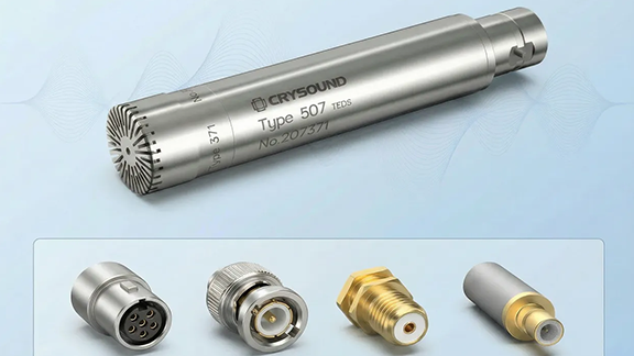
From the outside, a measurement microphone looks deceptively simple. But in real-world engineering, its interface options are surprisingly diverse: Lemo, BNC, Microdot, 10-32 UNF, M5, SMB… Many newcomers to acoustics ask questions like: Why can’t microphone interfaces be standardized? Why are cables often not interchangeable between microphones? What power and signal schemes are hidden behind different connectors? This article provides a structured overview of common measurement microphone interfaces, looking at physical connectors, powering methods, cable characteristics, and typical application-driven selection. Main Physical Interfaces for Measurement Microphones Below is a connector-by-connector summary, including the typical powering approach for each. Lemo (5-pin, 7-pin): The Classic Solution for Externally Polarized Microphones Lemo is a precision circular multi-pin connector and is the most common choice for externally polarized measurement microphones. The Lemo B series is widely used (e.g., 0B, 1B, 2B), and most standard measurement microphones adopt the Lemo 1B interface. Key Characteristics A multi-pin connector can carry multiple signals simultaneously, such as: Microphone output (analog signal) External polarization high voltage (typically 200 V) Preamplifier power supply Calibration/identification signals Additional benefits: Very reliable mechanical locking Well-suited for lab environments, metrology, and semi-anechoic chamber measurements where stability and traceability matter Notes on External Polarization Common polarization voltage is 200 V; some systems support switching between 0 V / 200 V Polarization voltage stability affects microphone sensitivity; in engineering practice, sensitivity variation is often treated as approximately proportional to voltage variation The preamplifier is typically powered separately (up to 120 V) but delivered via the same multi-pin connector Maximum output voltage can reach 50 Vp Includes pins for charge injection methods Separate output and ground paths help achieve lower noise In metrology labs, type testing, acoustic calibration, and high-precision semi-anechoic chamber work, the combination of “externally polarized microphone + Lemo multi-pin connector” is essentially a standard configuration. When not to use Lemo: Harsh environments with heavy contamination, oil exposure, and salt spray High costs of cables and connectors require careful trade-offs in field engineering applications BNC: The Most Common External Connector for IEPE Microphones Names like IEPE / ICP / CCP refer to the same general technology route: constant-current powering, where power and signal are transmitted on the same line (Constant Current Powering). In this system, the most common physical connector is the coaxial BNC. Interface and Powering Characteristics Coaxial structure, ideal for analog voltage transmission Bayonet lock (quick and reliable plug/unplug) Supports longer cable runs with good noise immunity Low cost and highly universal Typical IEPE Powering Parameters Constant current: 2–20 mA (common settings include 2 mA, 4 mA, 8 mA, etc.) Compliance voltage (supply capability): typically 18–24 V Maximum output voltage: generally around 8 Vp If the constant current is too low or the compliance voltage is insufficient, the maximum output signal swing is limited—directly affecting the maximum measurable SPL and the linear measurement range. In everyday testing such as engineering noise measurements, NVH, and environmental noise work, “IEPE microphone + BNC” has become the de facto standard. When not to use BNC: Applications requiring long-distance transmission of high-frequency signals, where signal attenuation becomes significant Applications involving frequent plugging and unplugging, to avoid an increased risk of poor electrical contact Microdot (10-32 UNF / M5): Lightweight Connectivity for Small Microphones Microdot is a threaded miniature coax connector widely used for small sensors (compact measurement microphones, accelerometers, etc.). It commonly uses a 10-32 UNF thread. What “10-32 UNF” Really Means This is simply an imperial fine-thread standard: Nominal diameter: 0.19 inch ≈ 4.826 mm Pitch: 1/32 inch ≈ 0.7938 mm Because 10-32 UNF is the typical thread used on Microdot connectors, the term “10-32 UNF” is often used informally to refer to the Microdot interface itself. What about M5? M5 is a metric thread standard: Nominal diameter: 5 mm Pitch: 0.8 mm Its dimensions are close to 10-32 UNF, and when tolerances are not extremely strict it can serve as a substitute—commonly seen in accelerometers or vibration microphones. Interface Characteristics Very compact; ideal for lightweight setups Threaded locking provides strong mechanical stability Commonly paired with IEPE powering Best for short runs and high-speed signal transmission When microphones must be placed in tight spaces, or where sensor mass/size is critical, Microdot is a common choice for compact, high-density installations. When not to use Microdot: Applications requiring quick connect/disconnect or frequent sensor replacement Use in systems with low constraints on installation space and requiring large-size connectors or high-power transmission, to avoid increased connection complexity and cost SMB (SubMiniature B): For High-Density Multi-Channel or Internal Connections SMB is a small “push-on” coaxial connector. Interface Characteristics Compact size supports high channel density Push-on structure enables fast connection Better high-frequency performance than BNC More suitable for semi-permanent internal wiring SMB is often best viewed as an engineering connector used inside equipment, rather than a field-plugging standard. When not to use Microdot: Applications involving frequent plugging and unplugging or repeated mechanical stress Use as a front-end connection interface for external devices, to avoid structural damage and reduced reliability Extended Interface Function: TEDS and Smart Identification In multi-channel and integrated systems, TEDS (Transducer Electronic Data Sheet) is increasingly common. By integrating a small memory chip into the sensor or cable, TEDS can store: Model and serial number Sensitivity Calibration date and other parameters Compatible front-end hardware or acquisition software can automatically read TEDS to: Identify the sensor type on each channel Load sensitivity and calibration coefficients automatically Reduce manual entry errors Save calibration time and labor At the connector level, TEDS is typically implemented by using certain pins in multi-pin Lemo connectors, or via overlay methods in specific BNC-based solutions. When planning an interface system, it’s wise to consider early on whether TEDS support is required. Why Are There So Many Interfaces? Connector diversity is best explained from three perspectives: Different Polarization and Powering Schemes Externally polarized microphones (≈ 200 V polarization) → better suited to multi-pin connectors like Lemo Prepolarized + IEPE systems → better suited to coaxial connectors like BNC / Microdot / SMB Different Scenarios and Priorities Laboratory / metrology: high stability, multiple signals in one cable, secure locking → Lemo Field engineering / environmental measurement: convenient wiring, strong universality → BNC + IEPE Miniaturization / high-density arrays: size and channel density first → Microdot / SMB Long Product Lifecycles and Backward Compatibility Measurement systems often have lifecycles of 10–20 years or more To avoid forcing users to replace large numbers of cables and front-end systems, manufacturers typically continue existing interface ecosystems Under long lifecycle constraints, “full unification” is often impractical and offers limited engineering return Typical Application Mapping (Quick Reference) Engineering noise, NVH, vibration/noise tests: BNC / MicrodotEasy wiring, many channels, low maintenance cost Precision lab measurement, type testing, metrology calibration: Lemo 7-pin / 5-pinSupports polarization HV and multiple signals; suitable for traceable high-precision measurement Acoustic arrays, multi-channel acquisition card systems: Microdot / SMBHigh channel density, compact wiring, easier system integration Long-term environmental noise monitoring systems: BNC / customized protected connectorsFocus on weather resistance, waterproofing, salt fog resistance, and stable long-distance transmission Conclusion The variety of measurement microphone interfaces is mainly the result of trade-offs between technology routes, application requirements, and historical compatibility—not simply a “lack of standards”. Taking NVH testing as an example: if an existing system uses BNC connectors to connect accelerometers, high-frequency signal attenuation and intermittent contact issues may occur in multi-channel array measurements. To improve connection reliability and signal quality, LEMO connectors with locking mechanisms and superior vibration resistance should be selected. After replacement, signal transmission stability is significantly improved, noise interference is reduced, and the consistency of test data is enhanced. You are welcome to learn more about microphone functions and hardware solutions on our website and use the “Get in touch” form to contact the CRYSOUND team.
How does your phone instantly and accurately connect to your earphones instead of someone else’s in a room full of Bluetooth devices? Why does your smart fitness band sync data exclusively to your phone app after a workout? This dedicated "one-to-one" connection relies on the Bluetooth 5.0 unicast mechanism. Its intelligence goes far beyond simple pairing—it lies in how it maintains a stable, efficient, and private wireless link with extremely low power consumption. Core Philosophy of Connection Strategy: Precision and Energy Efficiency Unlike Classic Bluetooth, which focuses on establishing a persistently online data channel, the Bluetooth 5.0 Low Energy (LE) unicast mode adopts a "wake-on-demand, instantaneous communication" design philosophy. It no longer maintains a continuous connection link but instead achieves efficient communication through a precise timing synchronization mechanism. After devices pair (e.g., a phone and a fitness band), they do not stay in a constantly connected state. Instead, they negotiate and establish a "connection interval," waking up synchronously only at predetermined moments to complete microsecond-level data exchange before immediately entering a deep sleep state. This mechanism allows devices to remain in an ultra-low power state for over 99% of the time, providing the core support for the long battery life (months to years) of IoT devices. Connection: Dynamic Coordination Under Precise Timing The establishment and maintenance of a Bluetooth 5.0 unicast connection rely on a precise timing coordination mechanism. The connection establishment process is as follows: Advertising and Scanning Phase: The peripheral device (e.g., earphone) sends advertising packets containing identity information at fixed intervals. The central device (e.g., phone) continuously scans on the advertising channels, searching for the target device. Connection Initiation Phase: The central device sends a connection request to the peripheral, which includes initial communication timing and suggested connection interval parameters. Connection Parameter Negotiation: This is the core of connection optimization. Beyond the connection interval, two other key parameters are negotiated: Slave Latency: When the slave device (e.g., fitness band) has no data to send, it can skip waking up for a specified number of connection interval cycles, thereby extending its sleep time. Supervision Timeout: A threshold for judging the connection state. If no valid communication occurs within this timeout period, the connection is considered lost, triggering reconnection or disconnection procedures. Connection Establishment and Maintenance: The master and slave devices switch to data channels, synchronizing their sleep and wake cycles according to the previously negotiated timing. This enables ultra-low power consumption while ensuring stable communication. New Product: CRY578 Bluetooth LE Audio Interface Empowering BLE Testing With the introduction of the new high-performance, low-complexity LC3 codec by the LE Audio standard, Bluetooth Low Energy (BLE) technology can now achieve stable transmission of high-quality stereo audio while maintaining its ultra-low power characteristics. Compared to traditional solutions, the LC3 codec can reduce bandwidth requirements by approximately 50% at the same audio quality or improve audio quality at the same bandwidth, effectively addressing the pain point of balancing low power consumption with high audio fidelity. In response to this technological trend, our newly launched CRY578 Bluetooth LE Audio Interface comprehensively supports audio performance testing for both Classic Bluetooth (BR/EDR) and Bluetooth Low Energy (BLE), covering core metrics such as frequency response, distortion, and audio latency. It is suitable for the R&D and quality inspection phases of various Bluetooth audio products, including TWS earphones, smart speakers, and wearable devices. For detailed specifications, application cases, or to inquire about trial opportunities for the CRY578, please fill out the “Get in touch” form below.
As smart devices continue to evolve, conversations about AI often revolve around visual perception, language models, or generative capabilities. Yet as devices become more immersive and more deeply embedded in our physical world, expectations are shifting—from machines that can see to machines that can truly hear. Many people still equate “hearing” with basic voice recognition, assuming it’s a solved problem. But as immersive audio and spatial experiences become core features of modern devices, sound is quietly emerging as the next major input channel for intelligent systems. We often ignore the ambient sounds around us—airflow from a computer, a washing machine spinning on the balcony, traffic rumbling outside the window. But if you close your eyes for a moment and focus, sound reveals far more than we usually notice. It travels through darkness, bypasses visual occlusion, and even reflects the shape of a space. For machines, this makes sound an invaluable source of environmental intelligence: footsteps, running water, engine noises—these carry information about people, objects, and events. This is where embodied intelligence comes into play: it enables devices not only to process speech, but also to understand the acoustic world. Figure 1. AI interpreting sound waves From Hearing to Orientation: Why IMUs Are Essential for Spatial Awareness Understanding external sounds is only one half of embodied intelligence. To truly comprehend space, a device must also understand itself—its orientation, posture, and movement in the environment. ● Hearing tells you what is happening. ● Self-orientation tells you where you are relative to what you hear. Imagine hearing a car approaching from your right. Without knowing which direction your head is turned, your brain cannot accurately determine where the car actually is. Machines face the same problem: auditory perception must be paired with spatial perception. Humans rely on the vestibular system inside the inner ear to estimate head movement and spatial orientation. Devices, on the other hand, rely on the IMU (Inertial Measurement Unit)—a tiny module that integrates gyroscopes, accelerometers, and sensor fusion algorithms to establish direction and posture. Today, IMUs power everything from spatial audio and gesture control to AR/VR head tracking and audiovisual synchronization. Figure 2. Immersive spatial audio experience Now imagine watching a movie or exploring an AR world: when you turn your head, you naturally expect the sound field to update instantly. If the IMU drifts or responds slowly, you may notice that: ● Sound lags behind your head movement. ● The perceived sound direction becomes inaccurate. ● Audio starts “wobbling” due to noisy readings. Even slight errors can break immersion, making the experience feel unnatural or even uncomfortable. This is why IMU accuracy and stability are critical—and why IMU testing has become a key part of the manufacturing process for AR/VR devices and advanced wearables. Making Perception Reliable: CRYSOUND’s IMU Testing Framework To ensure a consistent user experience, IMUs must undergo precise and standardized testing before devices leave the factory. Leveraging years of expertise in acoustic measurement, CRYSOUND has developed a comprehensive IMU performance testing framework designed to replicate “real-world head movements” inside the lab. At the core of this system is a three-axis motion platform capable of simulating the following motions: yaw (turning the head left or right), pitch (nodding up and down), and roll (tilting the head sideways). These cover the exact motion ranges most critical for spatial audio. Powered by high-precision servo motors, the platform achieves an absolute positioning accuracy of ±0.05° and repeatability of ±0.06°, enabling highly realistic motion reproduction. Figure 3. CRYSOUND three-axis IMU testing platform The testing workflow is fully automated: the operator simply places the device inside an RF-shielded chamber, and the system takes care of: ● Establishing Bluetooth connection ● Executing motion sequences ● Collecting raw IMU data ● Performing pass/fail analysis With efficient motion control and stable wireless communication, a full six-posture test for typical headphone products can be completed in about one minute per device—ideal for high-volume production lines. Although these processes happen behind the scenes, they directly shape the end-user experience: audio that moves naturally with your head, without delay, drift, or jitter—allowing immersion to feel seamless and real. As cloud computing and on-device processing continue to advance, the next generation of smart devices will increasingly differentiate themselves not by raw computing power, but by depth of perception. Sound perception and spatial orientation will form the backbone of that evolution. Combining auditory sensing with directional awareness—using IMUs to empower AI—marks a major step toward truly embodied intelligence. Only when a device can hear the environment, interpret spatial relationships, and understand its own motion can it genuinely “exist” in the physical world. If you’d like to learn more about how CRYSOUND’s IMU and acoustic testing solutions can support your AR/VR, headphone, or wearable projects, please fill out the “Get in touch” form on our website, and our team will get back to you shortly.
sound power
Under regulations such as the EU Machinery Noise Directive, more and more products—from toys and power tools to IT equipment—are required to declare their sound power level on labels and in documentation, rather than simply claiming they are “quiet enough.” For typical office devices like notebook computers, idle noise is often around 30 dB(A), while full-load operation can approach 40 dB(A). These figures are usually obtained from sound power measurements performed in accordance with ISO 3744 and related standards. Sound Pressure vs. Sound Power A noise source emits sound power, while what we measure with a microphone is sound pressure. Sound pressure varies with room size, reverberation, and microphone distance, whereas sound power is the source’s own “noise energy” and does not change with installation or environment. That makes sound power a better metric for external product noise specification. In simple terms: Sound power is the cause – the energy emitted by the source (unit: W / dB); Sound pressure is the effect – the sound pressure level we hear and measure (unit: Pa / dB). ISO 3744 defines how to do this in an “essentially free field over a reflecting plane”: arrange microphones around the source on an enveloping measurement surface, measure the sound pressure levels on that surface, then apply specified corrections and calculations to obtain stable, comparable sound power levels. Device Under Test: An Everyday Notebook Computer Assume our DUT is a 17-inch office notebook. The goal is to determine its A-weighted sound power level under different operating conditions (idle, office load, full load), in order to: Compare different cooling designs and fan control strategies; Provide standardized data for product documentation or compliance; Supply baseline data for sound quality engineering (for example, whether the fan noise is annoying). The test environment is a semi-anechoic room with a reflecting floor. The notebook is placed on the reflective plane, and multiple microphone positions are arranged around it (using a hemispherical frame or a regular grid). Overall, the setup satisfies ISO 3744 requirements for the measurement surface and environment. Measurement System: SonoDAQ Pro + OpenTest Sound Power Module On the hardware side, we use SonoDAQ Pro together with measurement microphones, arranged around the notebook according to the standard. OpenTest connects to SonoDAQ via the openDAQ protocol. In the channel setup interface, you select the channels to be used and configure parameters such as sensitivity and sampling rate. From Standard to Platform: Why Use OpenTest for Sound Power? OpenTest is CRYSOUND’s next-generation platform for acoustic and vibration testing. It supports three modes—Measure, Analysis, and Sequence—covering both R&D laboratories and repetitive production testing. For sound power applications, OpenTest implements a sound-pressure-based solution fully compliant with ISO 3744 (engineering method), and also covering ISO 3745 (precision method) and ISO 3746 (survey method). You can flexibly select the test grade according to the test environment and accuracy requirements. The platform includes dedicated sound power report templates that generate standards-compliant reports directly, avoiding repeated manual work in Excel. On the hardware side, OpenTest connects to multi-brand DAQ devices via openDAQ, ASIO, WASAPI, and NI-DAQmx, enabling unified management of CRYSOUND SonoDAQ, RME, NI and other systems. From a few channels for verification to large microphone arrays, everything can be handled within a single software platform. Three Steps: Running a Standardized ISO 3744 Sound Power Workflow Step 1: Parameter Setup and Environment Preparation After creating a new project in OpenTest: In the channel setup view, select the microphone channels to be used and configure sensitivity, sampling rate, frequency weighting, and other parameters. Switch to Measure > Sound Power and set the measurement parameters: Test method and measurement-surface-related parameters; Microphone position layout; Measurement time; Other parameters corresponding to ISO 3744. This step effectively turns the standard’s clauses into a reusable OpenTest scenario template. Step 2: Measure Background Noise First, Then Operating Noise According to ISO 3744, you must measure sound pressure levels on the same measurement surface with the device switched off and device running, in order to perform background noise corrections. In OpenTest, this is implemented as two clear operations: Acquire background noiseClick the background-noise acquisition icon in the toolbar. OpenTest records ambient noise for the preset duration.In the survey method, OpenTest updates LAeq for each channel once per second;In the engineering and precision methods, it updates the LAeq of each 1/3-octave band once per second. Acquire operating noiseAfter background acquisition, click the Test icon. OpenTest will:a. Record notebook operating noise for the preset duration;b. Update real-time sound pressure levels once per second;c. Automatically store the run as a data set for later replay and comparison. Step 3: From Multiple Measurements to One Standardized Report After completing multiple operating conditions (for example: idle, typical office work, full-load stress): In the data set view, select the records you want to compare and overlay them to observe sound power differences under different conditions; In the Data Selector, click the save icon to export the corresponding waveform files and CSV data tables for further processing or archiving; Click Report in the toolbar, fill in project and device information, select the data sets to include, adjust charts and tables, and export an Excel report with one click. The report includes measurement conditions, measurement surface, band or A-weighted sound power levels, background corrections, and other key information. It can be used directly for internal review or regulatory/customer submissions, following the same idea as other standardized sound power reporting solutions. From a Single Notebook Test to a Reusable Sound Power Platform Running an ISO 3744 sound power test on a notebook is just one example. More importantly: The standardized OpenTest scenario can be cloned for printers, home appliances, power tools, and many other products; Multi-channel microphone arrays and SonoDAQ hardware can be reused across projects within the same platform; The test workflow and report format are “locked in” by the software, making it easier to hand over, review, and audit across teams. If you are building or upgrading sound power testing capability, consider using ISO 3744 as the backbone and OpenTest as the platform that links environment, acquisition, analysis, and reporting into a repeatable chain—so each test is clearly traceable and more easily transformed from a one-off experiment into a lasting engineering asset. Visit www.opentest.com to learn more about OpenTest features and hardware solutions, or contact the CRYSOUND team by filling out the “Get in touch” form below.
In sound and vibration testing, flexibility is a decisive factor—especially when test requirements evolve rapidly. SonoDAQ, with its modular, scalable architecture, helps users easily manage everything from simple tests with a single device to complex, large-scale, multi-channel data acquisition. Whether in laboratory environments or industrial sites, SonoDAQ provides efficient, accurate data acquisition solutions, maximizing the adaptability and scalability of the system. Easy Testing with One Device, Scalable Expansion with Multiple Devices When testing requirements are modest, such as road tests or basic vibration testing, SonoDAQ Pro can easily meet the required number of channels with a single device. In this case, users only need one device to perform high-precision data acquisition, which is efficient and helps avoid unnecessary upfront hardware investment. However, as testing needs increase, especially in scenarios that require numerous sensors or synchronized multi-channel acquisition, SonoDAQ offers flexible expansion solutions. Users can connect multiple SonoDAQ Pro units in a daisy-chain or star topology to achieve large-scale data acquisition. For example, when conducting NVH testing or sound and vibration testing for large equipment, users can add more devices as needed, scaling up to hundreds of channels while ensuring high-precision synchronization across all devices. This scalability allows customers to avoid purchasing entirely new acquisition systems each time. By simply cascading existing SonoDAQ Pro units, they can easily cover more complex testing needs and avoid the common issues of device redundancy and high costs seen in traditional systems. Flexible Configuration to Meet Various Needs Even without large-scale acquisition needs, SonoDAQ remains highly flexible. With its modular design, users can easily adjust and reconfigure the system according to changing test requirements. For instance, if only temperature or strain signals are required, users can simply select the corresponding module and insert it into the chassis, without purchasing a new mainframe. This design makes SonoDAQ suitable for everything from simple laboratory tests to complex field tests. Users can expand the system as needed, without worrying about future expansion limits. Whether it's basic data acquisition or advanced signal analysis, SonoDAQ provides accurate, flexible data acquisition solutions, significantly enhancing testing efficiency and cost-effectiveness. Flexibility Brought by Modular Design The modular design of SonoDAQ is the core of its flexibility. Users can select different input modules, output modules, sensor interface modules, and more based on project requirements, and easily plug-and-play or upgrade them as needed. Whether it's adding more sensor channels or expanding with new functional modules, users can quickly implement changes by swapping modules, without affecting the normal operation of the existing system. This design ensures long-term device usability and enables SonoDAQ to adapt to ever-changing test requirements. When future requirements change, such as testing additional signal types (e.g., temperature, pressure, strain), SonoDAQ Pro can easily meet these new testing needs by simply swapping modules, allowing the overall system to continue running efficiently without the need for a full system overhaul. For example, an automotive manufacturer needs to perform NVH testing. Initially, they may only need 4–8 channels for in-car noise testing. In this case, engineers can use a single SonoDAQ Pro device to complete routine testing tasks. When they need to expand the testing scope and add more sensors (such as measuring vibration, strain, or temperature at different locations), they can simply daisy-chain multiple SonoDAQ Pro devices together. Through synchronization technology, they can ensure data consistency across all devices without redesigning the system or changing existing test procedures. Beyond automotive NVH, the same scalable architecture can be applied to aerospace components, industrial machinery, and even high-channel-count consumer electronics testing. Expand as Needed, Effortlessly Tackle Any Testing Challenge The flexible expansion capability of SonoDAQ allows it to scale from simple single-channel testing to large-scale multi-channel data acquisition. Whether it's for in-vehicle testing, industrial monitoring, or scientific research, SonoDAQ provides accurate, reliable data acquisition solutions. Its modular design and flexible system topology not only meet current needs but also enable quick adaptation to evolving testing scenarios in the future. Choosing SonoDAQ means moving away from fixed hardware configurations and instead adjusting the system based on needs, ensuring smooth, repeatable execution of every test. SonoDAQ is ready to transform your testing process—from simple single-device setups to large-scale, multi-channel systems. Contact us now: fill out the “Get in touch” form below, and our team will get back to you shortly.
SonoDAQ is the next-generation high-performance data acquisition system, specifically designed for sound and vibration testing. It features a modular architecture, making data acquisition more efficient and precise. From industrial environments to laboratory measurements, SonoDAQ meets the demands of high-precision data acquisition and provides seamless support for multi-channel synchronized data collection. Modular Design, Flexible to Adapt to Various Applications SonoDAQ adopts a completely new modular design, allowing for flexible configuration based on different needs. Whether you require a basic 4-channel setup or a large-scale system with hundreds of channels, SonoDAQ can easily accommodate both. You can select modules according to your project requirements and expand the system at any time, avoiding unnecessary costs. This flexibility is particularly well-suited for dynamic and evolving testing environments. High-Precision Synchronization Ensures the Accuracy of Test Results In sound and vibration testing, data accuracy is crucial. SonoDAQ is equipped with a 32-bit ADC and a sampling rate of up to 204.8 kHz. It ensures time synchronization between channels with a time error of less than 100 ns through PTP (IEEE 1588) and GPS synchronization. This level of synchronization precision allows you to obtain reliable and consistent data results, even in multi-channel, large-scale distributed acquisition systems. Flexible System Expansion with Multiple Network Topologies Another highlight of SonoDAQ is its powerful distributed acquisition capability. With various network connection methods like daisy chain and star topology, multiple devices can be easily integrated into the same acquisition system. Leveraging PTP (Precision Time Protocol) and GPS synchronization technology, SonoDAQ ensures nanosecond-level synchronization, providing data consistency across devices, whether for small-scale laboratory tests or large-scale field data collection. You can choose different system topologies based on your specific needs, offering flexibility for complex testing scenarios. Innovative Structural Design, the Ideal Choice for Field Applications SonoDAQ's frame is made using 5000t aluminum extrusion technology combined with carbon fiber-reinforced plastic, offering exceptional sturdiness while significantly reducing the device's weight. Additionally, SonoDAQ supports PoE power supply and hot-swappable batteries, ensuring efficient operation even in harsh environments and meeting the demands of long-duration continuous acquisition. Whether in the laboratory or on industrial sites, SonoDAQ delivers stable performance. Extensive Signal Compatibility, Expanding Your Testing Boundaries SonoDAQ supports a variety of signal inputs, including IEPE sensors, CAN bus, digital I/O, and other interface protocols. This allows it to meet a wide range of testing needs, from vibration monitoring to motor noise analysis. Whether you're conducting basic data acquisition or advanced signal analysis, SonoDAQ provides the precision and flexibility you require. Enhance Testing Efficiency, Making Data Acquisition Simpler With the accompanying OpenTest software, SonoDAQ allows you to monitor and analyze collected signals in real-time. OpenTest offers an intuitive interface and powerful data analysis features, making it easier to process and present test data. Additionally, SonoDAQ supports open protocols like ASIO and OpenDAQ, facilitating integration with other testing tools or software. SonoDAQ will help streamline your testing process, improve data acquisition efficiency, and provide precise measurements in various complex testing environments. Whether it's noise testing, vibration analysis, or complex sound power measurements, SonoDAQ is your ideal choice. Choose SonoDAQ today and bring revolutionary changes to your testing work! SonoDAQ is ready to transform your testing process — don’t wait to experience its power. Contact us now! Please fill out the 'Get in touch' form below, and we'll get back to you shortly!
With the development of technology and industry, acoustic technology has become increasingly mature and is now widely used in areas ranging from consumer electronics to aerospace, and from medical facilities to scientific research. In various industrial inspection scenarios, equipment maintenance, and fault diagnosis, acoustic imaging has become a fast and convenient tool. It can transform sound waves that are difficult for the human ear to detect into intuitive images, helping technicians quickly locate problems. CRYSOUND’s Acoustic Imaging products are designed for partial discharge detection, gas leak detection, mechanical fault detection, and more, and have been widely adopted in over ten industries, such as power distribution, automotive, and composites. So, how exactly do acoustic imaging systems work? This blog will explain the complete workflow of an acoustic imaging system—from sound wave acquisition to visual imaging—in a simple and easy-to-understand way. CRYSOUND Acoustic Imaging Camera Products 1. Sound Wave Acquisition: Capturing Invisible Sound Waves The core function of an acoustic imaging system is to capture sound waves, which are usually generated by vibrations, leaks, or malfunctions during equipment operation. When sound waves propagate through the air, they cause air molecules to vibrate, forming pressure waves. Acoustic imaging systems receive these pressure waves through a built-in microphone array (usually composed of multiple high-sensitivity microphones). Each microphone can independently capture the frequency, intensity, and phase information of the sound wave, like taking a 'fingerprint' of the sound. For example, when a motor malfunctions, the wear of its internal bearings generates high-frequency vibrations. These vibrations propagate through the air and are captured by the microphone array of the acoustic imaging system. By analyzing these acoustic signals, technicians can initially determine the type and location of the fault. Gas Leak Detection Mechanical Faults Detection Partial Discharge Detection 2. Signal Processing: From Raw Data to Useful Information The acquired acoustic signals are analog signals and need to be converted into digital signals by an analog-to-digital converter (ADC). These digital signals then enter the signal processing unit for a series of complex calculations. These calculations include: Noise Reduction: Using digital filtering techniques, environmental noise and other interference signals are removed, retaining useful acoustic information. Beamforming: Utilizing the spatial distribution of the microphone array, algorithms calculate the direction and distance of the sound source. This process is similar to using multiple ears to locate the sound source. Spectrum Analysis: The acoustic signal is decomposed into components of different frequencies, and the intensity of each frequency component is analyzed to determine the nature of the sound source (e.g., mechanical faults, leaks, etc.). After these processes, the raw acoustic signal is transformed into useful information containing the sound source’s location, intensity, and frequency characteristics. 3. Visual Imaging: Converting Sound into Images The processed acoustic data needs to be presented to the user in an intuitive way. Acoustic imaging cameras visualize sound through the following steps: Data Mapping: Mapping the location information of the sound source onto two-dimensional or three-dimensional space to form a sound source distribution map. Typically, an acoustic imaging camera uses color to represent sound wave intensity: red or yellow indicates a strong sound source, and blue or green indicates a weak sound source. Image Overlay: Overlaying the sound source distribution map with a visible-light image or infrared image to form a composite image. This allows users to see the physical appearance of the equipment and the distribution of sound sources on the same image, thus quickly locating problem areas. Real-time Display: Acoustic imaging cameras typically provide real-time imaging capabilities, dynamically displaying changes in sound sources. This is extremely useful for monitoring equipment operating status and diagnosing faults. 4. Application Scenarios: A Wide Range of Uses The working principle of acoustic imaging makes it widely applicable in multiple fields. In the industrial field, acoustic imaging cameras can be used to detect mechanical faults, gas leaks, and electrical problems in equipment. For example, by analyzing the sound waves of a transformer during operation, it is possible to determine whether there is internal discharge or loosening. 5. Technical Advantages: High Efficiency, Precision, and Non-Contact The working principle of acoustic imaging systems gives them the following technical advantages: High Efficiency: Acoustic imaging cameras can quickly scan large areas and display the distribution of sound sources in real time, greatly improving detection efficiency. Precision: Through advanced signal processing algorithms, acoustic imaging cameras can accurately locate the position and intensity of sound sources, with errors typically within a few centimeters. Non-Contact: Acoustic imaging cameras do not require contact with the device under test, avoiding potential damage or interference from traditional detection methods. Conclusion Acoustic imaging systems transform invisible sound into intuitive images by capturing sound waves, processing signals, and visualizing images, providing a powerful tool for fault diagnosis and equipment maintenance. Although their working principle involves complex signal processing algorithms, the core logic is simple and easy to understand: from sound wave acquisition to visual imaging, every step is aimed at converting sound into useful information. With the continuous development of technology, acoustic imaging technology will continue to demonstrate its unique value in more fields. If you are interested in CRYSOUND’s acoustic imaging solutions or would like to discuss your specific application, please fill out the 'Get in touch' form below and our team will be happy to assist you.