Browse Authors

Blogs

AR Glasses Production-Line Testing Upgrade – Multi-Station Audio & VPU Solution

As the AR glasses market transitions from proof-of-concept to large-scale commercialization, product capabilities in audio and haptic interaction continue to expand, driving increased demands for production-line testing. With key modules such as audio and VPU (Vibration Processing Units), AR glass production-line testing is evolving from simple functional validation to consistency control aimed at enhancing real-world user experience. Based on actual mass production project experience, this article introduces audio and VPU testing solutions for different workstations, with a focus on free-field audio testing, VPU deployment, and fixture design, providing practical reference for scaling AR glasses manufacturing. Accelerating Market Expansion of AR Glasses and New Trends in Production-Line Testing As smart glasses products mature, their functional boundaries are expanding rapidly. According to various industry reports, the shipment volume and investment scale of AR glasses continue to increase, with the market shifting from concept validation to commercialization. Products driven by companies like Meta are increasingly capable of supporting voice interaction, calls, notifications, and recording, supplementing functions traditionally carried out by smartphones and earphones. This shift has transformed AR glasses from a low-frequency conceptual product into a high-frequency wearable interaction terminal. Consequently, audio capabilities have become a core component of the smart glasses experience, directly impacting voice interaction and call quality. At the same time, vibration and haptic feedback have been introduced to enhance interaction confirmation and user perception. As these capabilities become commonplace in mass-produced products, production-line testing is no longer just focused on whether basic functions work but is now required to handle multiple critical capabilities, such as audio and VPU, simultaneously. This shift presents new challenges for upgrading production-line testing solutions. Audio Testing Solutions for Multi-Station Production Lines Audio is one of the most directly influential functions on the user experience of AR glasses, and its production-line testing needs to balance accuracy, consistency, and production efficiency. In a multi-station production environment, audio testing is often distributed across several workstations depending on the assembly phase. At the temple or frame workstations, audio testing focuses more on validating the basic performance of individual microphones or speakers, ensuring that key components meet the requirements early in the assembly process and avoiding costly rework later on in the process. At the final assembly workstation, the focus shifts to overall audio performance and system-level coordination. While different workstations focus on different aspects, the fixture positioning, acoustic environment control, and testing process design need to maintain consistent logic throughout. CRYSOUND’s AR glass audio testing solutions are designed to address this need, with a unified testing architecture that allows flexible deployment across different workstations while maintaining stable and consistent results. The solutions can be divided into the following two types, meeting the aesthetic and UPH requirements of different production lines. Drawer-Type Single-Unit (1-to-1) Easy automation integration Standing operation for convenient loading and unloading Simultaneous testing of SPK and MIC (airtightness), supporting multi-MIC scenarios Serial testing for left and right SPK, parallel testing for multiple MICs Supports Bluetooth, USB ADB, and Wi-Fi ADB communication Average cycle time (CT): 100s | UPH: 36 Clamshell Dual-Unit (1-to-2) Parallel dual-unit testing for improved efficiency Ergonomic seated operation design Simultaneous testing of SPK and MIC (airtightness), supporting multi-MIC scenarios Serial testing for left and right SPK (single box), parallel testing for multiple MICs Supports Bluetooth, USB ADB, and Wi-Fi ADB communication Average cycle time (CT): 150s | UPH: 70 Speaker EQ in AR Glasses: From Pressure Field to Free Field In traditional earphone products, speaker EQ is usually built in a relatively stable pressure-field environment, where ear coupling and wearing style have a well-controlled impact on the acoustic environment. In contrast, AR glasses typically use open structures for the speakers, with no sealed cavity between the driver and the ear, making their acoustic performance closer to free-field characteristics. This structural difference makes the frequency response of AR glasses speakers more sensitive to sound radiation direction, structural reflections, and wearing posture, and dictates that their EQ strategy cannot simply follow earphone product experience. In the production-line testing and tuning process, the speaker EQ for AR glasses needs to be evaluated and validated under free-field conditions. Due to the open acoustic structure, the frequency response is more susceptible to structural reflections, assembly tolerances, and variations in wearing posture, making it difficult to rely solely on hardware consistency to ensure stable listening across different products. By introducing EQ tuning, these systemic deviations can be compensated without changing the structural design, improving the consistency of audio performance during mass production. The focus of the testing solution is not to pursue idealized sound quality, but rather to capture real acoustic differences under stable and repeatable free-field testing conditions, providing reliable data for EQ parameter validation. CRYSOUND supports customized EQ algorithms. In one mass production project, speaker EQ calibration was introduced at the final test station under free-field conditions, and the results were accepted by the customer, validating the applicability and practical significance of this solution for glasses products. VPU Testing Solutions for AR/Smart Glasses Why AR Glasses Include VPU (Vibration Processing Unit) As AR/smart glasses increasingly support voice interaction, calls, and notifications, relying on audio feedback alone is no longer enough. In noisy environments, privacy-sensitive scenarios, or with low-volume prompts, users need a feedback method that does not disturb others but is sufficiently clear. This is where VPU is introduced. Unlike traditional earphones, glasses are not always tightly coupled to the ear, making audio prompts more susceptible to environmental noise. By utilizing vibration or haptic feedback, the system can convey status confirmations, interaction responses, or notifications to users without increasing volume or relying on screens. Therefore, VPU becomes a key component for supplementing or even replacing some audio feedback in AR glasses. Primary Roles of VPU in AR Glasses In current mass-produced smart glasses designs, VPU typically serves the following functions: Interaction confirmation feedback: such as successful voice wake-up, completed command recognition, or the start/stop of recording or photo taking. Silent notifications: vibrational feedback in scenarios where audio prompts are unsuitable. Enhanced experience: boosting interaction certainty and immersion when combined with audio feedback. These functions have made VPU an essential capability in the AR glasses interaction experience, rather than just an optional feature. Typical VPU Placement in AR Glasses (Why in the Nose Bridge/Pads) Structurally, VPU is typically located near the nose bridge or nose pads for three main reasons: Proximity to sensitive body areas: The nose bridge is sensitive to small vibrations, providing high feedback efficiency. Stable and consistent coupling: Compared to the temples, the nose bridge has a more stable and consistent contact with the face, ensuring better vibration transmission. Does not interfere with audio device layout: Avoids interference with speakers and microphones in the temple region. Therefore, during production-line testing, VPU is often tested as an independent target, requiring dedicated verification at the frame or final assembly stage. VPU Testing Implementation and Consistency Control on the Production Line Based on the functional positioning and structural characteristics of VPU in AR glasses, VPU testing is typically scheduled based on the product form and assembly progress in mass production. In some cases, testing may even be moved earlier in the process to identify potential VPU issues before they are exacerbated in subsequent assembly stages. It is important to note that production-line testing environments differ fundamentally from laboratory validation environments. In laboratory testing, VPU is typically tested as a standalone component under simplified conditions and higher excitation levels (e.g., 1g). However, in production-line environments, the VPU is already integrated into the frame or complete product, requiring excitation conditions that closely mimic those of real-world wearing scenarios. In practice, production-line VPU testing typically takes place in the 0.1g–0.2g, 100–2kHz excitation range, verifying consistency in VPU performance under realistic physical conditions. CRYSOUND’s AR glasses VPU production-line testing solution uses the CRY6151B Electro-Acoustic Analyzer as the testing and analysis platform. The vibration table provides stable excitation, and the product VPU synchronizes vibration response signals with a reference accelerometer. Software analysis evaluates key parameters such as frequency response (FR) and total harmonic distortion (THD).This test architecture balances testing effectiveness and production-line throughput, meeting the deployment needs for VPU testing at different stations. Compared to audio testing, VPU testing is more sensitive to testing configurations and fixture design, with less room for error and greater difficulty in consistency control. Based on experience from multiple projects, fixture design must fully account for structural differences in locations such as the nose bridge and nose pads. It is important to prioritize materials and contact methods that facilitate vibration transmission, and to design standardized fixture shapes that keep the fixture's center of gravity aligned with the vibration table's working plane, minimizing the introduction of additional variables at the structural level. By following these design principles, the stability and repeatability of VPU test results can be improved in a production-line environment, providing reliable support for validating the product's VPU capabilities. From Functional Testing to Experience Constraints In AR glasses production lines, the role of testing is evolving. In the past, audio or vibration modules were more likely to be treated as independent functions, with the goal of confirming whether they were "functional." However, with the current form of the product, these modules directly influence voice interaction, wearing comfort, and overall experience. As a result, the test results now serve as a prerequisite for the overall product performance. For example, audio and VPU modules are no longer just performance verification items; they now play a role in the consistency control of the user experience. The interaction between audio performance, vibration feedback, and structural assembly means that production-line testing needs to identify potential issues that could affect the experience in advance, rather than just filtering out problems at the final inspection stage. This change is pushing test strategies from "functional pass" to "experience control." If you’d like to learn more about AR glasses audio testing solutions—or discuss your blade process and inspection targets—please use the “Get in touch” form below. Our team can share recommended settings and an on-site workflow tailored to your production conditions.

Octave-Band Analysis Guide: FFT Binning vs. Filter Bank Method

Octave-band analysis can be implemented in two fundamentally different ways: FFT binning (integrating PSD/FFT bins into 1/1- and 1/3-octave bands) and a true octave filter bank (standards-oriented bandpass filters + RMS/Leq averaging). In this post, we compare how the two methods work, where their results match, where they diverge (scaling, window ENBW, band-edge weighting, latency, transient response), and how OpenTest supports both for acoustics, NVH, and compliance measurement. For a detailed explanation of the concepts, read this → Octave-Band Analysis: The Mathematical and Engineering Rationale Octave-band filter banks (true octave / CPB filter bank) Parallel bandpass filters + energy detector + time averaging A filter-bank (true octave) analyzer typically: Design a bandpass filter H_b(z) (or H_b(s)) for each band center frequency. Run filters in parallel to obtain band signals y_b(t). Compute band mean-square/power and apply time averaging to output band levels. To be comparable across instruments, filter magnitude responses must satisfy IEC/ANSI tolerance masks (class) for the specified filter set. [1][3] IIR vs FIR: why IIR (cascaded biquads) is common in practice IIR advantages: lower order for a given roll-off, lower compute, good for real-time/embedded; stable when implemented as SOS/biquads. FIR advantages: linear phase is possible (useful when waveform shape matters); design/verification can be more straightforward. For band-level outputs, phase is usually not the primary concern, so IIR filter banks are common. Multirate processing: the “secret weapon” of CPB filter banks Low-frequency CPB bands are very narrow. Implementing them at the full sampling rate is inefficient. A common strategy is to group bands by octave and downsample for low-frequency groups: Low-pass then decimate (e.g., by 2 per octave) for lower-frequency groups. Implement the corresponding bandpass filters at the reduced sampling rate. Ensure adequate anti-aliasing before decimation. Time averaging / time weighting: band levels are statistics, not instantaneous values Band levels typically require time averaging. Common options include block RMS, exponential averaging, or Leq (energy-equivalent level). In sound level meter contexts, IEC 61672-1 defines Fast/Slow time weightings (Fast ~125 ms, Slow ~1 s). [5][6] Engineering implication: different time constants produce different readings, so time weighting must be stated in reports. How to validate that a filter bank behaves “like the standard” Sine sweep: verify passband behavior and adjacent-band isolation; observe time delay effects. Pink/white noise: verify average band levels and variance/stabilization time; check effective bandwidth behavior. Impulse/step: examine ringing and time response (critical for transient use). Cross-check against a known compliant reference instrument/implementation. From band definitions to compliant digital filters: an end-to-end workflow (conceptual) Choose the band system: base-10/base-2, the fraction 1/b (commonly b=3), generate exact fm and f1/f2. Choose performance target: which standard edition and which class/mask tolerance? Choose filter structure: IIR SOS for real-time; FIR or forward-backward filtering if phase/zero-phase is required. Design each bandpass: map f1/f2 into the digital domain correctly (e.g., pre-warp for bilinear transform). Implement multirate if needed: decimate for low-frequency groups with sufficient anti-alias filtering. Verify: magnitude response vs mask; noise tests for effective bandwidth; sweep/impulse tests for time response. Calibrate and report: units and reference quantities, averaging/time weighting, method details. Time response explained: group delay, ringing, and averaging all shape readings A band-level analyzer is a time-domain system (filter → energy detector → smoother), so readings are governed by multiple time scales: Filter group delay: how late events appear in each band. Filter ringing/decay: how long a short pulse “rings” within a band. Energy averaging/time weighting: the time resolution vs fluctuation of the output level. Thus, for transients (impacts, start/stop events, sweeps), different compliant implementations can yield different peak levels and time tracks—consistent with ANSI’s caution. [3] Rule of thumb: for steady-state contributions, use longer averaging for stability; for transient localization, shorten averaging but accept higher variability and lock down algorithm details. Common real-time pitfalls Forgetting anti-aliasing in the decimation chain: low-frequency bands become contaminated by aliasing. Numerical instability of high-Q low-frequency IIR sections: use SOS/biquads and sufficient precision. Averaging in dB: always average in energy/mean-square, then convert to dB. Assuming band energies must sum exactly to total energy: standard filters are not necessarily power-complementary; verify using standard-consistent criteria instead. Octave-Band Filter Bank Analysis in OpenTest OpenTest supports octave-band analysis using a filter-bank approach:1) Connect the device, such as SonoDAQ Pro2) Select the channels and adjust the parameter settings. For an external microphone, enable IEPE and switch to acoustic signal measurement.3) In the Octave-Band Analysis section under Measurement Mode, choose the IEC 61260-1 algorithm. It supports real-time analysis, linear averaging, exponential averaging, and peak hold.4) After configuring the parameters, click the Test button to start the measurement.5) A single recording can be analyzed simultaneously in 1/1-octave, 1/3-octave, 1/6-octave, 1/12-octave, 1/24-octave, and 1/24-octave bands. Figure 1: Octave-Band Filter Bank Analysis in OpenTest FFT binning and FFT synthesis FFT binning: convert a narrowband spectrum into CPB band integrals Estimate spectrum (single FFT, Welch PSD, or STFT). Integrate/sum within each octave/fractional-octave band to obtain band power. This is common in software/offline work because a single FFT provides high-resolution spectrum that can be re-binned into any band system (1/1, 1/3, 1/12, …). Key challenge #1: FFT scaling and window corrections After an FFT, scaling depends on your definitions: 1/N normalization, amplitude vs power vs PSD, one-sided vs two-sided spectrum, and windowing. For noise measurements, ENBW is crucial; ignoring it can introduce systematic offsets. [7] A practical PSD normalization (periodogram form) # convert to one-sided PSD: multiply by 2 except DC (and Nyquist if present) This yields PSD in units of (input unit)²/Hz and supports energy consistency checks by integrating PSD over frequency. Two quick self-checks for scaling White noise check: generate noise with known variance σ²; integrate one-sided PSD over 0..fs/2 and recover ≈σ² (accounting for the ×2 rule). Pure tone check: generate a sine with amplitude A (RMS=A/√2); integrating spectral energy should recover ≈A²/2 (subject to leakage and window choice). If both checks pass, your FFT scaling is likely correct; then partial-bin weighting and octave binning become meaningful. Key challenge #2: band edges rarely align to bins → partial-bin weighting Hard include/exclude decisions at band edges cause step-like errors, especially at low frequency where bands are narrow. Use overlap-based weighting (Section 4.2.4) for the boundary bins. Does zero-padding solve edge misalignment? (common misconception) Zero-padding interpolates the displayed spectrum but does not improve true frequency resolution (which is set by the original window length). It can reduce visual stair-stepping but cannot turn 1–2-bin low-frequency bands into reliable band-level estimates. Fundamental fixes are longer windows or multirate processing/filter banks. Key challenge #3: time–frequency trade-off (window length sets low-frequency accuracy and delay) FFT resolution is Δf = fs/N. Low-frequency 1/3-octave bands can be only a few Hz wide, so achieving enough bins per band requires very large N, increasing latency and smoothing transients. Root cause: 1/3 octave is constant-Q, but STFT uses constant-Δf bins In CPB, band width scales with frequency (Δf_band ∝ f, constant-Q). In STFT, bin spacing is constant (Δf_bin constant). Therefore low-frequency CPB needs extremely fine Δf_bin (long windows), while high frequency is over-resolved. Solution routes: long-window STFT vs multirate STFT vs CQT/wavelets Long-window STFT: simplest, but high latency and transient smearing. Multirate STFT: downsample low-frequency content and FFT at lower fs, similar in spirit to multirate filter banks. Constant-Q transform (CQT) / wavelets: naturally logarithmic resolution, but matching IEC/ANSI masks requires extra calibration/validation. [4] For compliance measurements, standards-oriented filter banks are preferred; for research/feature extraction, CQT/wavelets can be attractive. FFT synthesis: constructing per-band filtering in the frequency domain FFT synthesis pushes the FFT approach closer to a filter bank: Define a frequency-domain weight W_b[k] per band (brick-wall or smooth/mask-like). Compute Y_b[k] = X[k]·W_b[k] and IFFT to get y_b[n]. Compute band RMS/averages from y_b[n]. It can easily implement zero-phase (non-causal) filtering. For strict IEC/ANSI matching, W_b and normalization must be carefully designed and validated. Making FFT synthesis stream-like: OLA, dual windows, and amplitude normalization To output continuous time signals per band, use overlap-add (OLA): frame, window, FFT, apply W_b, IFFT, synthesis window, and OLA. Choose analysis/synthesis windows to satisfy COLA (constant overlap-add) conditions (e.g., Hann with 50% overlap) to avoid periodic level modulation. If the goal is to match standard filters, how should W_b be chosen? W_b[k] depends on what you want to match: Match brick-wall integration: W_b is hard 0/1 within [f1,f2]. Match IEC/ANSI filter behavior: |W_b(f)| approximates the standard mask and effective bandwidth (matches ∫|W_b|²). Match energy complementarity for reconstruction: design Σ_b |W_b(f)|² ≈ 1 (Section 7.6). You typically cannot satisfy all three perfectly at once; define your priority (compliance vs decomposition/reconstruction) up front. Energy-conserving frequency-domain filter banks: why Σ|W_b|² matters If you want band energies to sum to total energy (within numerical error), a common design aims for approximate power complementarity: IEC/ANSI masks do not necessarily enforce strict complementarity, so don’t assume exact additivity in compliance contexts. Welch/averaging strategies: how to make FFT band levels stable Use Welch averaging (segment, window, overlap, average power spectra). Average in the power domain (|X|² or PSD), then convert to dB. For non-stationary signals, consider STFT to obtain time–band matrices. Report window type, overlap, averaging count, and ENBW/CG treatment. FFT-Binning Analysis in OpenTest OpenTest supports octave-band analysis based on FFT binning:1) Connect the device, such asSonoDAQ Pro2) Select the channels and adjust the parameter settings. For an external microphone, enable IEPE and switch to acoustic signal measurement.3) In the Octave-Band Analysis section under Measurement Mode, choose the FFT-based algorithm.4) A single recording can be analyzed simultaneously in 1/1-octave, 1/3-octave, 1/6-octave, 1/12-octave, and 1/24-octave bands. Figure 2: FFT-Binning Octave-Band Analysis in OpenTest Filter-bank vs FFT/FFT synthesis: differences, equivalence conditions, and trade-offs A comparison table DimensionFilter-bank (True Octave / CPB)FFT binning / FFT synthesisStandards complianceEasier to match IEC/ANSI magnitude masks; mainstream for hardware instruments. [1][3]Hard binning behaves like band integration; matching masks requires extra weighting or standard-compliant digital filters.Real-time / latencyCausal real-time possible; latency set by filter order and averaging.Block processing adds at least one window length of delay; low-frequency resolution often forces longer windows.Transient responseContinuous output but affected by group delay/ringing; different compliant implementations may differ. [3]Set by STFT windowing; transients are smeared by windows and sensitive to window type/length.Leakage & correctionsControlled via filter design; leakage can be managed.Strongly depends on window and ENBW/scaling; edge-bin misalignment needs partial weighting. [7]InterpretabilityRMS after bandpass filtering—aligned with sound level meters and analyzers.Spectrum estimation + binning—more statistical; interpretation depends on window/averaging settings.ComputationMany filters in parallel; multirate can reduce cost.One FFT can serve all bands; efficient for offline/batch.Phase & reconstructionIIR is typically nonlinear phase (fine for levels).Frequency weights can be zero-phase; reconstruction needs attention to complementarity and transitions. When do both methods give (almost) the same answers? Band-averaged results typically agree closely when: You compare averaged band levels (not transient peak tracks). The signal is approximately stationary and the observation time is long enough. FFT resolution is fine enough that each band contains enough bins (especially at the lowest band). FFT scaling is correct (one-sided handling, Δf, window U, ENBW/CG where needed). Partial-bin weighting is used at band edges. Why differences grow for transients and short events Differences are driven by mismatched time scales: filter banks have band-dependent group delay and ringing but continuous output; STFT uses a fixed window that sets both frequency resolution and time smoothing. If event duration is comparable to the window length or filter impulse response, results depend strongly on implementation details. Error budget: where mismatches usually come from (and how to locate them quickly) Wrong averaging/combination in dB: must average and sum in the energy domain. Inconsistent FFT scaling: 1/N conventions, one-sided vs two-sided, Δf, window normalization U. Missing window corrections: ENBW for noise; coherent gain/leakage for tones. Using nominal frequencies to compute edges instead of exact definitions. No partial-bin weighting at band boundaries (especially harmful at low frequency). Multirate/anti-alias issues in filter banks. Different averaging time constants/windows between methods. True method differences: brick-wall binning vs standard filter skirts/roll-off imply systematic offsets. A strong debugging approach: first match total mean-square using white noise (scaling/ENBW/partial-bin), then validate band centers and adjacent-band isolation using swept sines or tones. Engineering checklist: make 1/3-octave analysis correct, stable, and reproducible Choose a method: compliance → filter bank; offline statistics → FFT binning For regulations/type testing/instrument comparability: prefer IEC/ANSI-compliant filter banks and report standard edition and class. [1][3] For offline processing, large datasets, or flexible band definitions: FFT binning can be efficient, but scaling and boundary weighting must be rigorous. If you need per-band time-domain signals (modulation, envelope, etc.): consider FFT synthesis or explicit filter banks. Selecting FFT parameters from the lowest band (example) Example: fs=48 kHz, lowest band of interest is 20 Hz (1/3 octave). Its bandwidth is only a few Hz. If you want at least M=10 bins per band, you may need Δf_bin ≤ bandwidth/10, implying a very large N (e.g., ~100k points; 2^17=131072). This illustrates why real-time compliance often favors filter banks. Typical mistakes that prevent results from matching Summing magnitude |X| instead of power |X|² or PSD. Averaging in dB instead of in linear power/mean-square. Ignoring ENBW/window scaling for noise. [7] Computing band edges from nominal frequencies. Not stating time weighting/averaging conventions (Fast/Slow/Leq). [5][6] Recommended validation flow (regardless of implementation) Tone-at-center test (or sweep): verify that energy peaks in the correct band and adjacent-band rejection behaves as expected. White/pink noise: verify expected spectral shape in band levels and assess stability/averaging time. Cross-implementation comparison: compare your implementation with a known reference on identical signals; isolate scaling vs definition vs filter-skirt differences. Record and freeze parameters (band definition, windowing, averaging) in the test report. Reproducibility checklist: include these in reports so others can recompute your levels Band definition: base-10 or base-2? b in 1/b? exact vs nominal used for computation? reference frequency fr? Implementation: standard filter bank (IIR/FIR, multirate) vs FFT binning/synthesis; software/library versions. Sampling/preprocessing: fs, detrending/DC removal, anti-alias filtering, resampling. Time averaging: Leq / block RMS / exponential; time constants, block size, overlap, averaging frames; Fast/Slow context if relevant. FFT details (if used): window type, N, hop, zero-padding, PSD normalization, one-sided handling, ENBW/CG, partial-bin weighting. Calibration/units: input units and reference quantities (e.g., 20 µPa), sensor calibration factors and dates. Output definition: RMS vs peak vs band power; 10log vs 20log conventions; any band aggregation steps. If you remember one line: document “band definition + time averaging + FFT scaling/window treatment (if any)”. Most disputes disappear. Quick formulas and numeric example (ready for code/report) Base-10 one-third-octave constants G = 10^(3/10) ≈ 1.995262 r = 10^(1/10) ≈ 1.258925 # adjacent center-frequency ratio k = 10^(1/20) ≈ 1.122018 # edge multiplier about center f1 = fm / k f2 = fm * k Example: the 1 kHz one-third-octave band fm = 1000 Hz f1 = 1000 / 1.122018 ≈ 891.25 Hz f2 = 1000 * 1.122018 ≈ 1122.02 Hz Δf ≈ 230.77 Hz Q ≈ 4.33 OpenTest integrates both methods. Download and get started now -> or fill out the form below ↓ to schedule a live demo. Explore more features and application stories at www.opentest.com. References [1] IEC 61260-1:2014 PDF sample (iTeh): https://cdn.standards.iteh.ai/samples/13383/3c4ae3e762b540cc8111744cb8f0ae8e/IEC-61260-1-2014.pdf [3] ANSI S1.11-2004 preview PDF (ASA/ANSI): https://webstore.ansi.org/preview-pages/ASA/preview_ANSI%2BS1.11-2004.pdf [4] HEAD acoustics Application Note: FFT - 1/n-Octave Analysis - Wavelet (filter bank description): https://cdn.head-acoustics.com/fileadmin/data/global/Application-Notes/SVP/FFT-nthOctave-Wavelet_e.pdf [5] IEC 61672-1:2013 (IEC page): https://webstore.iec.ch/en/publication/5708 [6] NTi Audio Know-how: Fast/Slow time weighting (IEC 61672-1 context): https://www.nti-audio.com/en/support/know-how/fast-slow-impulse-time-weighting-what-do-they-mean [7] MathWorks: ENBW definition example: https://www.mathworks.com/help/signal/ref/enbw.html

Octave-Band Analysis: The Mathematical and Engineering Rationale

Octave-band analysis converts detailed spectra into standardized 1/1- and 1/3-octave bands using constant-percentage bandwidth on a logarithmic frequency axis. In this post, we explain the mathematical basis of CPB, why IEC 61260-1 and ANSI S1.11 define octave bands the way they do, and how band levels are computed in practice (FFT binning vs. filter-bank RMS). The goal: repeatable, comparable results for acoustics, NVH, and compliance measurements. What is octave-band analysis, and what problem does it solve? Octave-band analysis is a family of spectrum analysis methods that partition the frequency axis on a logarithmic scale into band-pass bands. Each band has a constant ratio between its upper and lower cut-off frequencies (constant percentage bandwidth, CPB). Within each band we ignore fine line-spectrum details and focus on total energy / RMS (or power) in that band. In other words, it is not “what happens at every 1 Hz,” but “how energy is distributed across equal relative bandwidths.” This representation naturally matches human hearing and many engineering systems, whose frequency resolution is often closer to a relative (log) scale than a fixed-Hz scale. It is a common reporting format required by many standards: room acoustics parameters, sound insulation ratings, environmental noise, machinery noise, wind/road noise, etc., often use 1/3-octave bands. From linear Hz to log frequency: why CPB looks more like an engineering language Using equal-width frequency bins (e.g., every 10 Hz) to accumulate energy leads to inconsistent behavior across the spectrum: At low frequencies, a 10 Hz bin may be too wide and can smear details. At high frequencies, a 10 Hz bin may be too narrow, giving higher variance and less stable estimates for random noise. In contrast, CPB bandwidth grows with frequency (Δf ∝ f). Each band covers a similar relative change, improving stability and repeatability—important for standardized testing. A visual intuition: bandwidth increases on a linear axis, but is uniform on a log axis Figure 1: the same 1/3-octave bands plotted on a linear frequency axis—bandwidth appears larger at high frequencies Each horizontal segment represents a 1/3-octave band [f1, f2]; the short vertical mark is the band center frequency fm. On a linear axis, higher-frequency bands look wider. Figure 2: the same bands on a logarithmic frequency axis—bands become evenly spaced (the essence of CPB) Once the horizontal axis is logarithmic, these bands appear equal-width/equal-spacing; this is exactly what “constant percentage bandwidth” means. These two figures capture the core idea: octave-band analysis uses equal steps on a log-frequency scale, not equal steps in Hz. Standards and terminology: what do IEC/ANSI/ISO systems actually specify? In practice, “doing 1/3-octave analysis” is constrained by more than just band edges. Standards specify (or strongly imply): how center frequencies are defined (exact vs nominal), the octave ratio definition (base-10 vs base-2), filter tolerances/classes, and even the measurement/averaging conventions used to form band levels. IEC 61260-1:2014 highlights: base-10 ratio, reference frequency, and center-frequency formulas IEC 61260-1:2014 is a key specification for octave-band and fractional-octave-band filters. It adopts a base-10 design: the octave frequency ratio is G = 10^(3/10) ≈ 1.99526 (very close to 2, but not exactly 2). The reference frequency is fr = 1000 Hz. It provides formulas for the exact mid-band (center) frequencies and specifies that the geometric mean of band-edge frequencies equals the center frequency. [1] Key formulas (rearranged from the standard): [1] If the fractional denominator b is odd (e.g., 1, 3, 5, ...): If b is even (e.g., 2, 4, 6, ...): And always: Why does the even-b case look “half-step shifted”? Intuitively, the center-frequency grid is evenly spaced on log(f). When b is even, IEC chooses a half-step offset relative to fr so that band edges align more neatly in common reporting conventions. In practice, a robust implementation is to generate the exact fm sequence using the standard’s formula, then compute edges via f1 = fm / G^(1/(2b)) and f2 = fm * G^(1/(2b)), and only then label bands by the usual nominal frequencies. View the data with OpenTest (IEC 61260-1 Octave-Band Analysis) -> Band edges, center frequency, and the bandwidth designator b Standards commonly use 1/b as the “bandwidth designator”: 1/1 is one octave, 1/3 is one-third octave, etc. [1] Once (G, b, fr) are chosen, the entire band set (centers and edges) is fixed mathematically. Exact vs nominal: why two “center frequencies” appear for the same band “Exact” center frequencies are used for mathematically consistent definitions and filter design; “nominal” values are used for labeling and reporting. [1] ISO 266:1997 defines preferred frequencies for acoustics measurements based on ISO 3 preferred-number series (R10), referenced to 1000 Hz. [2] As a result, the exact geometric sequence is typically labeled with familiar nominal values such as: 20, 25, 31.5, 40, 50, 63, 80, 100, 125, 160, …, 1k, 1.25k, 1.6k, 2k, 2.5k, 3.15k, …, 20k. Implementation tip: compute edges from exact frequencies; only round/display as nominal. This avoids drifting away from the standard. Base-10 vs base-2: why standards don’t insist on an exact 2:1 octave Although “octave” is often thought of as 2:1, IEC 61260-1 specifies base-10 (G=10^(3/10)) rather than G=2. Key motivations include: Alignment with decimal preferred-number series (ISO 266 is tied to R10). [2] International consistency: IEC 61260-1:2014 specifies base-10 and notes that base-2 designs are less likely to remain compliant far from the reference frequency. [1] In base-10, one-third octave corresponds to 10^(1/10) ≈ 1.258925 (also interpretable as 1/10 decade), which yields a clean mapping: 10 one-third-octave bands per decade. “10 one-third-octave bands = 1 decade”: why this matters With base-10 one-third-octave spacing, each step multiplies frequency by r = 10^(1/10). Therefore: 10 consecutive 1/3-octave bands multiply frequency by exactly 10 (one decade). This matches ISO 266/R10 conventions and simplifies tables, plotting, and communication. Standardization values readability and consistency as much as raw mathematical purity. Figure 3: Base-10 one-third-octave spacing—10 equal ratio steps per decade (×10 in frequency) ANSI S1.11 / ANSI/ASA S1.11: tolerance classes and a transient-signal caution ANSI S1.11 (and later ANSI/ASA adoptions aligned with IEC 61260-1) specify performance requirements for filter sets and analyzers, including tolerance classes (often class 0/1/2 depending on edition). [3][4] A practical caution in ANSI documents: for transient signals, different compliant implementations can produce different results. [3] This highlights that time response (group delay, ringing, averaging time constants) matters for transient analysis. What do class/mask/effective bandwidth actually control? “I used 1/3-octave bands” is not just about nominal band edges. Standards aim to ensure different instruments/algorithms yield comparable results by constraining: Frequency spacing: center-frequency sequence and edge definitions (base-10, exact/nominal, f1/f2). Magnitude response tolerance (mask): allowable ripple near passband and required attenuation away from center. Energy consistency for broadband noise: constraints on effective bandwidth so band levels are comparable across implementations. Effective bandwidth matters because real filters are not ideal brick walls. For broadband noise, the output energy depends on ∫|H(f)|^2 S(f)df. Differences in passband ripple, skirts, and roll-off can cause systematic offsets. Standards constrain effective bandwidth to keep such offsets within acceptable limits. [1][3][4] The transient caution is not a contradiction: masks mainly constrain steady-state frequency-domain behavior, while transients depend on phase/group delay, ringing, and time averaging. [3] Mathematics: band definitions, bandwidth, Q, and band indexing CPB and equal spacing on a log axis CPB is equivalent to equal-width spacing in log-frequency. If u = log(f), then every band spans a fixed Δu. Many spectra (e.g., 1/f-type) look smoother and statistically more stable in log frequency. Band-edge formulas from the geometric-mean definition (general 1/b form) IEC defines the center frequency as the geometric mean of the edges: fm = sqrt(f1 f2). [1] For 1/b octave bands, the edge ratio is typically f2/f1 = G^(1/b), where G is the octave ratio. Then: For base-10 one-third octave (b=3): G=10^(3/10). Adjacent center ratio is r = G^(1/3) = 10^(1/10) ≈ 1.258925; edge multiplier is k = 10^(1/20) ≈ 1.122018. Q-factor and resolution: octave analysis is constant-Q analysis Define Q = fm / (f2 − f1). For CPB bands, Δf = f2 − f1 scales with fm, so Q depends only on b and G (not on frequency). Quick reference (base-10, fr=1000 Hz): Fractional-octaveBand ratio f2/f1Relative bandwidth Δf/fmQ = fm/Δf1/11.9952620.7045921.4191/21.4125380.3471072.8811/31.2589250.2307684.3331/61.1220180.1151938.6811/121.0592540.05757317.369 Interpretation: for 1/3 octave, Q≈4.33 and each band is about 23% wide relative to its center. Finer bands (1/6, 1/12) give higher resolution but higher variance for random noise and typically require longer averaging. Band numbering (integer index) and formulaic enumeration Implementations often use an integer band index x. In IEC, x appears directly in the center-frequency formula: fm = fr * G^(x/b). [1] This provides a stable way to enumerate all bands covering a target frequency range and ensures contiguous, standard-consistent edges. For base-10: so and you can invert as Figure 4: Q factor for common fractional-octave bandwidths (base-10 definition) Two meanings of “1/3 octave”: base-2 vs base-10—do not mix them Some literature uses base-2: adjacent centers are 2^(1/3). IEC 61260-1 and much modern acoustics practice use base-10: adjacent centers are 10^(1/10). A quick check: if nominal centers look like 1.0k → 1.25k → 1.6k → 2.0k (R10 style), it is likely base-10. Mathematical definition of band levels: from PSD integration to dB reporting Continuous-frequency view: integrate PSD within the band Octave-band level is essentially the integral of power spectral density over a frequency band. For sound pressure p(t): For vibration (velocity/acceleration), the same logic applies with different units and reference quantities. Key point: because dB is logarithmic, any summation or averaging must be performed in the linear power/mean-square domain first. Two discrete implementations: filter-bank RMS vs FFT/PSD binning Filter-bank method: y_b(t)=BandPass_b{x(t)}, then compute mean(y_b^2) as band mean-square (optionally with time averaging). FFT/PSD binning method: estimate S_pp(f) (e.g., via periodogram/Welch), then numerically integrate/sum bins within [f1,f2]. For long, stationary signals, averaged results can be very close. For transients, sweeps, and short events, they often differ. Be explicit about what spectrum you have: magnitude, power, PSD (and dB/Hz) Magnitude spectrum |X(f)|: amplitude units (e.g., Pa), useful for tones/harmonics. Power spectrum |X(f)|²: mean-square units (Pa²). Power spectral density (PSD): mean-square per Hz (Pa²/Hz), most common for noise. Because octave-band levels represent band mean-square/power, you must end up integrating/summing in Pa² (or analogous) regardless of starting representation. Frequency resolution and one-sided spectra: Δf, 0..fs/2, and the “×2” rule FFT bin spacing is Δf = fs/N. A typical discrete approximation is: If you use a one-sided spectrum (0..fs/2), to conserve energy you typically multiply all non-DC and non-Nyquist bins by 2 (because negative-frequency power is folded into the positive side). Different software handles these conventions differently, so align definitions before comparing results. Window corrections: coherent gain (tones) vs ENBW (noise) are different Windowing reduces spectral leakage but changes scaling: For tone amplitude: correct by coherent gain (CG), often CG = sum(w)/N. For broadband noise/PSD: correct by equivalent noise bandwidth (ENBW), e.g., ENBW = fs·sum(w²)/(sum(w))². [9] CG controls peak amplitude; ENBW controls average noise-floor area. Octave-band levels are energy statistics and are more sensitive to ENBW. WindowCoherent Gain (CG)ENBW (bins)Rectangular1.0001.000Hann0.5001.500Hamming0.5401.363Blackman0.4201.727 Partial-bin weighting: what to do when band edges do not align to FFT bins Band edges rarely land exactly on bin frequencies. Treat PSD as approximately constant within each bin of width Δf, and weight boundary bins by their overlap fraction: This produces smoother, more physically consistent band levels when N or band edges change. Figure 5: Partial-bin weighting schematic when band edges do not align with FFT bins A unifying formula: both methods compute ∫|H_b(f)|² S_xx(f) df Both filter-bank and PSD binning can be written as: Brick-wall binning corresponds to |H_b|² being 1 inside [f1,f2] and 0 outside. A true standards-compliant filter has a roll-off and ripple, which is why standards constrain masks and effective bandwidth. Band aggregation: composing 1-octave from 1/3-octave, and forming total levels Under ideal partitioning and energy accounting: Three adjacent 1/3-octave bands can be combined to approximate one full octave band. Summing all band energies over a covered range yields the total energy. Always combine in the energy domain. If L_i are band levels in dB, energies are E_i = 10^(L_i/10). Then: IEC 61260-1 notes that fractional-octave results can be combined to form wider-band levels. [1] Effective bandwidth: why standards specify it Real filters are not ideal rectangles. For white noise (constant PSD S0), output mean-square is: For non-white spectra such as pink noise (PSD ~ 1/f), standards may define normalized effective bandwidth with weighting to maintain comparability across typical engineering noise spectra. [1] Practical implication: FFT “hard-binning” implicitly assumes a brick-wall filter with B_eff = (f2 − f1). A compliant octave filter has skirts, so B_eff can differ slightly (and by class). To match results, either approximate the standard’s |H(f)|² in the frequency domain or document the methodological difference. Why 1/3 octave is favored (math + perception + engineering trade-offs) Information density is “just right”: finer than 1 octave, steadier than very fine fractions A single octave band can be too coarse and hide spectral shape; very fine fractions (e.g., 1/12, 1/24) can be unstable and expensive: Higher estimator variance for random noise (each band captures less energy). More computation and higher reporting burden. Often more detail than regulations or rating schemes need. One-third octave is the classic compromise: enough resolution for engineering insight, stable enough for standardized measurements, and broadly supported by instruments and software. Psychoacoustics: critical bands in mid-frequencies are close to 1/3 octave Many psychoacoustics references describe ~24 critical bands across the audible range, and in the mid-frequency region the critical-bandwidth is often similar to a 1/3-octave bandwidth. [7][8] This makes 1/3 octave a natural intermediate representation for problems tied to perceived sound, while still being more standardized than Bark/ERB scales. Direct standards/application pull: many workflows mandate 1/3 octave I/O Once major standards define inputs/outputs in 1/3 octave, ecosystems (instruments, software, reporting templates) converge around it. Examples: Building acoustics ratings: ISO 717-1 references one-third-octave bands for single-number quantity calculations. [5] Room acoustics parameters (e.g., reverberation time) are commonly reported in octave/one-third-octave bands (ISO 3382 series). [6] Extra base-10 benefits: R10 tables, 10 bands/decade, readability 10 bands per decade: multiplying frequency by 10 corresponds to exactly 10 one-third-octave steps (very clean for log plots). R10 preferred numbers: 1.00, 1.25, 1.60, 2.00, 2.50, 3.15, 4.00, 5.00, 6.30, 8.00 (×10^n) are widely recognized and easy to communicate. Compared with base-2, decimal labeling is less awkward and cross-standard ambiguity is reduced. Octave-band analysis is typically implemented using either FFT binning or a filter bank. Keep reading -> Octave-Band Analysis Guide: FFT Binning vs. Filter Bank OpenTest integrates both methods. Download and get started now -> or fill out the form below ↓ to schedule a live demo. Explore more features and application stories at www.opentest.com. References [1] IEC 61260-1:2014 PDF sample (iTeh): https://cdn.standards.iteh.ai/samples/13383/3c4ae3e762b540cc8111744cb8f0ae8e/IEC-61260-1-2014.pdf [2] ISO 266:1997, Acoustics - Preferred frequencies (ISO): https://www.iso.org/obp/ui/ [3] ANSI S1.11-2004 preview PDF (ASA/ANSI): https://webstore.ansi.org/preview-pages/ASA/preview_ANSI%2BS1.11-2004.pdf [4] ANSI/ASA S1.11-2014/Part 1 / IEC 61260-1:2014 preview: https://webstore.ansi.org/preview-pages/ASA/preview_ANSI%2BASA%2BS1.11-2014%2BPart%2B1%2BIEC%2B61260-1-2014%2B%28R2019%29.pdf [5] ISO 717-1:2020 abstract (mentions one-third-octave usage): https://www.iso.org/standard/77435.html [6] ISO 3382-2:2008 abstract (room acoustics parameters): https://www.iso.org/standard/36201.html [7] Ansys Help: Bark scale and critical bands (mentions midrange close to third octave): https://ansyshelp.ansys.com/public/Views/Secured/corp/v252/en/Sound_SAS_UG/Sound/UG_SAS/bark_scale_and_critical_bands_179506.html [8] Simon Fraser University Sonic Studio Handbook: Critical Band and Critical Bandwidth: https://www.sfu.ca/sonic-studio-webdav/cmns/Handbook5/handbook/Critical_Band.html [9] MathWorks: ENBW definition example: https://www.mathworks.com/help/signal/ref/enbw.html

SonoDAQ Enclosure Coating Hardness Test

In real DAQ use, enclosure durability and scratch resistance directly affect service life and maintenance cost. This article shares a pencil hardness scratch test on the SonoDAQ top cover (PC + carbon fiber) and compares it with a typical laptop enclosure. The results show how the enclosure performs from 2H to 5H and why the surface finish helps it hold up in daily handling. How Scratch Resistance Affects DAQ Use When choosing a DAQ front end, engineers usually look first at the specs—sample rate, dynamic range, synchronization accuracy, channel count… But after a few years of real use, many realize that enclosure reliability and scratch resistance can be just as important to the system’s service life and day-to-day experience. For soundand vibration test equipment, this is even more obvious. Typical SonoDAQ applications include NVH road tests, on-site industrial measurements, and long-term outdoor or semi-outdoor acquisition, where the device often has to: be carried frequently, loaded into vehicles, or fixed on fixtures or test benches; be moved between lab desks, instrument carts, and tool cases; remain in close contact with other metal equipment, screwdrivers, laptops, and more. In such environments, a housing that scratches easily not only looks worn, but can also drive up maintenance and replacement costs. To better reflect daily handling, we ran a pencil-hardness scratch test on the SonoDAQ front-end upper cover and used a common laptop enclosure as a reference. Test Setup The test was performed strictly in accordance with ISO 15184:2020, and was intended to evaluate the scratch resistance of the UV-cured coating on the outer surface of the SonoDAQ front-end upper cover. Samples SampleDescriptionA — SonoDAQ top coverMaterial: PC + carbon-fiber plate (top/bottom covers), with an internal aluminum frame and corner protection.B — Typical laptop enclosureMaterial: Plastic/metal housing with a sprayed coating. This test follows the pencil hardness test approach. Pencils of different hardness grades were used to scratch the enclosure surface under consistent contact conditions, and the surface was inspected for any scratches visible to the naked eye. Test Tools Pencil hardness tester, additional weights can be added as required. Pencils: hardness grades 2H, 3H, 4H, and 5H. Procedure Insert the pencil into the pencil hardness tester at a 45° angle, with a total load of 750 g (equivalent to applying 7.5 N to the coating surface). For each pencil hardness grade, scratch the enclosure surface three times and check whether any visible scratches appear. Keep the scratch length and applied force as consistent as possible to ensure comparability across hardness grades. Results Criteria Whether visible scratches appear; Whether the surface gloss changes noticeably. Results From the results, we could see that the front-end enclosure showed different levels of scratch resistance under different pencil grades. To further validate durability, we ran the same pencil hardness test on a typical laptop enclosure. Laptop housings are usually plastic or metal and also have a painted surface. We used the same method as for the DAQ unit: 2H Pencil: SonoDAQ ProTypical Laptop Conclusion: Neither the SonoDAQ enclosure nor the laptop enclosure showed any obvious scratches; visually there was almost no change. 3H Pencil: SonoDAQ ProTypical Laptop Conclusion: Neither the SonoDAQ enclosure nor the laptop enclosure showed any obvious scratches; visually there was almost no change. 4H Pencil: SonoDAQ ProTypical Laptop Conclusion: At 4H, the SonoDAQ enclosure still showed no visible scratches; in contrast, the laptop enclosure exhibited clearly visible scuffs, essentially reaching the upper limit of its scratch resistance. 5H Pencil: SonoDAQ Pro Conclusion: At 5H, light scratches began to appear on the SonoDAQ enclosure, indicating it was approaching its scratch-resistance limit. Note that the pencil hardness test is primarily a relative comparison of scratch resistance between enclosures; it does not represent a material’s absolute hardness or long-term wear life. However, for assessing whether a surface is “easy to scratch” in everyday use, it is a very direct method. If we translate the pencil grades into typical real-world scenarios: Accidental rubbing from most keys, equipment edges, and tools usually falls in the 2H-3H range; 4H-5H corresponds to harder, sharper, and more forceful scratching—often with some deliberate pressure. At 4H, the SonoDAQ enclosure is still difficult to mark, and it only shows slight scratching at 5H. This means that during normal handling, loading, installation, and daily use, the enclosure is not easy to scratch. Why It Holds Up The SonoDAQ front-end enclosure uses a PC + carbon-fiber composite, which provides good mechanical strength and toughness. On top of that, the surface is finished with a spray-and-bake paint process plus a UV-cured top layer, which plays a key role in: Increasing surface hardness and improving scratch resistance; Improving corrosion resistance and environmental robustness; Balancing durability with a premium look and feel. For instrumentation, “harder” is not always “better.” The right design balances scratch resistance, impact resistance, weight, and long-term reliability. As the results show, SonoDAQ’s enclosure is durable enough for real-world use. For more information on SonoDAQ features, application scenarios, and typical configurations, please fill out the Get in touch form below to contact the CRYSOUND team. We will provide selection recommendations and support based on your test requirements.

Differences Between Measurement Microphones and Regular Microphones

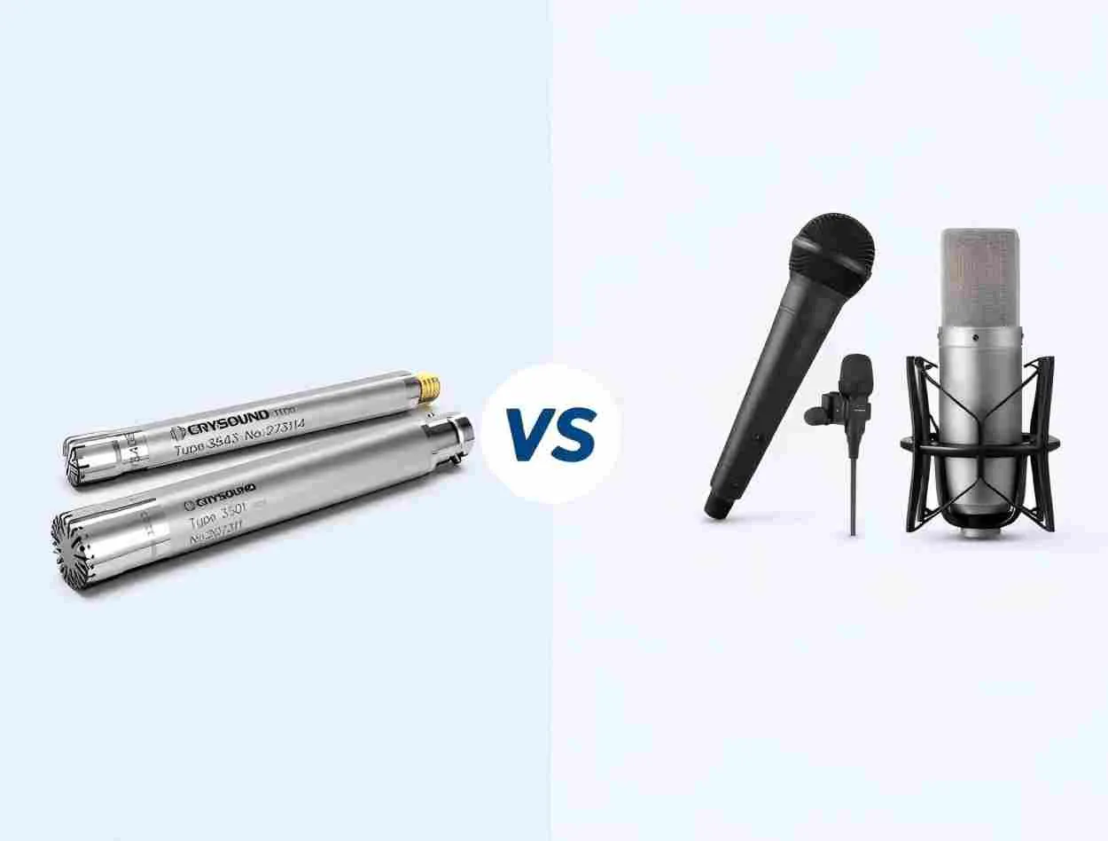
Across acoustics testing, product R&D, environmental noise monitoring, and NVH analysis, simply “capturing sound” isn’t the goal—accurate sound measurement is. A measurement microphone is engineered for repeatable, traceable, and quantifiable results, so your data stays comparable across devices, labs, and time. In this post, we explain what a measurement microphone is and how it differs from a regular microphone, based on real-world acoustic measurement workflows. What Is a Measurement Microphone? A measurement microphone is a high-precision acoustic transducer designed to measure sound pressure accurately. Its purpose is not to make audio “sound good,” but to be truthful, calibratable, and repeatable. A typical measurement microphone is engineered to provide: Known and stable sensitivity (e.g., mV/Pa), so its electrical output can be converted into sound pressure (Pa) or sound pressure level (dB). Controlled, near-ideal frequency response (as flat as possible under specified sound-field conditions) for accurate multi-band measurement. Excellent linearity and wide dynamic range, maintaining low distortion from very low noise floors to high SPL environments. Traceable calibration capability, working with acoustic calibrators or pistonphones to manage measurement uncertainty and maintain a reliable measurement chain. Environmental stability, minimizing drift due to temperature, humidity, static pressure, and long-term aging—critical for both lab and field use. In short: a measurement microphone is the front-end sensor of a metrology-grade measurement chain, where the output must meaningfully represent true sound pressure in a defined sound field. What Is a Regular Microphone? Most microphones people encounter daily—conference mics, phone mics, streaming mics, stage mics, and studio mics—are built for audio capture and production. They typically prioritize: Speech clarity and pleasing timbre Wind/plosive resistance and usability Directivity and feedback control System compatibility, size, durability, and cost Many regular microphones are intentionally not flat. For example, they may boost the vocal presence band, roll off low frequencies, or apply built-in processing such as noise reduction, AGC (automatic gain control), and limiting. These features can be great for “good sound,” but they can severely compromise measurement accuracy. The Core Difference: Different Goals, Different Design Philosophy Measurement Accuracy vs. Pleasant Sound Measurement microphones aim to represent true sound pressure with accuracy, repeatability, and traceability. Regular microphones aim to produce usable or pleasant audio, where tonal shaping is often desired. Calibration and Traceability: Quantifiable vs. Hard to Quantify Measurement microphones are designed to support periodic calibration: Regular microphones are typically treated as functional audio devices—specs may be provided, but traceable metrology calibration is rarely central to their usage. Quick Comparison Table DimensionMeasurement MicrophoneRegular MicrophonePrimary GoalAccurate, traceable measurementAudio capture and sound qualityFrequency ResponseControlled & defined (free/pressure/diffuse field)Tuned for application; may be intentionally shapedCalibrationDesigned for calibration and uncertainty managementTypically not traceable or routinely calibratedLinearity/Dynamic RangeEmphasizes wide range, low distortionLimiting/compression/processingKey SpecsSensitivity, equivalent noise, max SPL, phase, driftSensitivity, directivity, timbre, ease of useTypical Use CasesAcoustics testing, compliance, R&D, NVH, monitoringMeetings, streaming, recording, stage, calls Why Do You Need a Measurement Microphone? If your work involves any of the following, a measurement microphone is often essential: Acoustic product development: loudspeaker/headphone response & distortion, spatial acoustics, array localization NVH engineering: cabin noise, transfer path analysis, order tracking Environmental/industrial noise monitoring: long-term stability and verifiable SPL logging Standards and compliance testing: traceable results and reproducible procedures across labs Acoustic material and silencer evaluation: impedance tubes, reverberation chambers, anechoic measurements In these scenarios, the real problem is rarely “can you record sound?” The real question is: can you trust the dB value? If your work involves any of the scenarios above, CRYSOUND’s measurement microphones are specifically designed for these high-standard applications, delivering stable, reliable, and consistent measurement data to fully meet the demands of such use cases. Conclusion: Measurement Turns Sound into Reliable Data A regular microphone helps you hear. A measurement microphone helps you verify. When you need to put acoustics into engineering reports, standards, and closed-loop product improvement, a measurement microphone is the foundation that makes results defensible. To learn more about microphone functions and measurement hardware solutions, visit our website—and if you’d like to talk to the CRYSOUND team, please fill out the “Get in touch” form.

Panelized PCBA Test for Multi-Product Lines

CRYSOUND’s PCBA testing solution integrates RF and audio performance validation within a 1-to-8 parallel architecture, enabling synchronized electrical, RF, audio, and power testing. This unified platform enhances PCBA test efficiency and adaptability for TWS, smart speakers, and wearables, driving cost-effective, high-volume production with streamlined integration. Industry Pain Points: Challenges of Traditional PCBA Testing in Multi-Category Production As smart hardware products diversify and iteration cycles shorten, traditional automated testing equipment increasingly exposes limitations—especially in cross-category production scenarios: Low space utilization: Traditional testers are typically customized for a single product category. Power testing for smart speakers, low-power testing for smart glasses, and RF testing for earbuds often require separate dedicated equipment, leading to excessive floor space usage and high expansion costs. High labor costs: Single-board testing systems require dedicated operators for calibration and supervision. Different operating logics across devices increase training costs, while peak production periods often rely on temporary staffing, causing labor costs to scale directly with output. Low production efficiency: Testing processes are largely serial. Panelized boards must be transferred between multiple stations, and special procedures—such as multi-channel audio testing for smart speakers—further extend cycle times, making it difficult to meet delivery demands. These issues ultimately trap manufacturers in an operational dilemma of “higher output equals higher costs, and product changes equal line downtime,” limiting responsiveness and profit growth. Core Advantages: An Integrated Solution for Multi-Scenario Applications Leveraging a mature technical architecture and extensive industry experience, the CRYSOUND panelized PCBA testing solution abandons the traditional “single-function, single-application” design philosophy. Instead, it addresses real-world multi-category production needs to optimize both testing efficiency and cost control. Fully Integrated Design with Over 50% Space Optimization The solution integrates key testing functions—including electrical performance, RF validation, audio inspection, and power stability testing—into a single system, forming a one-stop testing workflow: Smart speaker applications: Integrated multi-channel audio testing and high-power stability modules eliminate the need for separate acoustic chambers and power validation benches. The system occupies only 25 m², saving 58% of space compared to traditional distributed layouts. Smart glasses applications: Designed for compact PCBA form factors, the system focuses on precise low-power current measurement and short-range RF validation, reducing damage risks caused by multi-station transfers. TWS/OWS earbud applications: RF, audio, and current parameter testing are completed within a single station. The 8-channel parallel testing architecture supports efficient panelized testing cycles. Through functional integration, a single system can replace 3–4 traditional dedicated testers, significantly improving workshop space utilization and enabling flexible capacity expansion. Intelligent Operations and Maintenance: Approximately 60% Labor Cost Reduction With a standardized user interface, the solution supports semi-unattended testing operations: Automated process control: After manual loading, the system automatically completes barcode registration, synchronized multi-module testing, and real-time data uploads. Abnormal conditions trigger tiered alarm mechanisms without requiring full-time supervision. Unified operating logic: All systems use a standardized human–machine interface. Operators can manage multi-category testing after a single training session, significantly reducing training costs and operational errors. Improved maintenance efficiency: One technician can manage four systems simultaneously, compared with the traditional ratio of one operator for two machines—resulting in a 200% increase in labor efficiency. Parallel Testing Architecture: Doubling Production Throughput By breaking through the bottleneck of serial testing, the multi-channel parallel testing design allows different test modules to operate simultaneously, dramatically reducing panelized board test cycles: Smart speakers: Parallel multi-channel audio and RF testing increases throughput from approximately 150 boards/hour to 300 boards/hour or more. TWS/OWS earbuds: The 8-channel parallel configuration achieves stable throughput of over 400 boards/hour, representing an efficiency improvement of approximately 150% compared with traditional single-channel systems. This approach eliminates the need to “add more machines to increase capacity,” enabling manufacturers to meet peak-order demands while optimizing cost efficiency. Standardized Technical Assurance: Precision and Reliability All core test modules undergo strict calibration and validation, meeting recognized industry standards: Equipped with RF test modules, MBT electrical performance modules, and audio loopback closed-loop testing units, supporting precise testing of mainstream chipsets from Qualcomm, BES, JieLi, and others. Testing accuracy complies with IPC-A-610 PCBA acceptability standards. RF shielding effectiveness reaches ≥70 dB within 700 MHz–6 GHz, audio distortion remains <1.5% within 100 Hz–10 kHz, and electrical measurement accuracy is controlled within ±0.5% of full scale. Test data can be stored in multiple formats, enabling full traceability from pre-test to post-test stages and meeting ISO 9001 quality management system requirements. Cost Advantages: Quantified Results Across Multiple Dimensions The CRYSOUND solution delivers sustainable cost advantages across equipment procurement, operations, and quality control: Equipment investment: Integrated design reduces the number of dedicated testers required, lowering initial equipment investment by over 30% for multi-category production. Operational costs: Optimized space utilization and reduced staffing requirements lower rental and labor expenses, saving RMB 150,000–300,000 per system annually. Quality costs: Integrated testing minimizes handling damage during panel transfers. For lightweight boards such as those used in smart glasses, damage rates drop by 30%, while precise testing and data traceability keep defect rates below 2%, representing a 40%+ reduction compared with traditional approaches. Case Studies: Efficiency Upgrades in Multi-Category Production The following cases are based on anonymized production data from real customers and demonstrate actual deployment results: Case 1: Mid-Sized TWS Earphone ODM (Monthly Output: 500,000 Units) Initial challenges: Four traditional test lines deployed in an 800 m² workshop, each requiring four operators. Single-line throughput was approximately 200 boards/hour, creating delivery pressure during peak seasons. Results after implementation: Four traditional lines were consolidated into two CRYSOUND test lines, freeing 200 m² of space for expansion. Each line required only 1.5 operators, saving RMB 45,000 per month in labor costs. Throughput per line increased to 400 boards/hour, doubling total monthly capacity to 1 million units, while delivery cycles shortened from 15 days to 10 days. Core value: Space utilization improved by 25%, labor costs reduced by 37.5%, and capacity increased by 24%. Case 2: Smart Speaker Brand Factory (Monthly Output: 150,000 Units) Initial challenges: Multi-channel audio testing and RF testing were separated into two stations, occupying 60 m². High-power testing defect rates reached 1.2%, mainly due to board damage during transfers. Results after implementation: The integrated system occupied only 25 m², saving 35 m² of production space. Eliminating multi-station transfers reduced handling-related defect rates to 0.5%, preventing the loss of approximately 1,000 units per month. Core value: Space usage reduced by 50%, changeover efficiency improved by 25%, and transfer-related defect rates decreased by 31.8%. The solution is now running stably across 10+ factories and 30+ production lines. Key Differences vs. Traditional Automated Test Equipment Comparison DimensionTraditional Automated EquipmentCRYSOUND Integrated Testing SolutionFunctional adaptabilitySingle-category customization; multiple systems required for cross-category productionIntegrated multi-scenario testing covering earbuds, speakers, and glassesChangeover efficiencyNo standardized process; line downtime up to 32 hoursParameterized configuration; downtime reduced to 4 hoursSpace utilizationDispersed single-function layouts with low efficiencyIntegrated design saving 50%+ spaceInitial investmentHigh due to multiple equipment purchasesOver 30% savings through integration CRYSOUND replaces the traditional “function-driven equipment” model with a “production-driven system” approach, enabling a shift from “adapting production to equipment” to “designing equipment around production.” Choose CRYSOUND Panelized PCBA Testing for Certainty in Quality and Efficiency As competition in smart wearable and consumer electronics markets intensifies, quality consistency and delivery speed are decisive factors. The CRYSOUND 1-to-8 PCBA comprehensive testing system is more than a piece of equipment—it is a complete solution for strengthening production-line competitiveness. By ensuring reliable wireless performance, optimized power consumption, and built-in safety validation for every PCBA leaving the factory, CRYSOUND helps manufacturers maintain full confidence and control over product quality, even at large-scale production volumes. If you’d like to learn more about PCBA testing—or discuss your blade process and inspection targets—please use the “Get in touch” form below. Our team can share recommended settings and an on-site workflow tailored to your production conditions.

Visualized Vacuum Leak Testing for Trains

Negative-pressure airtightness is critical for high-speed train car bodies, and even minor leaks can lead to rework or delivery risks. This article presents a case from Changchun where CRYSOUND’s CRY8124 Acoustic Imaging Camera was used to quickly, intuitively, and verifiably pinpoint leaks on a carbon-fiber train car body shell, showcasing the CRY8124’s application in vacuum leak detection for carbon-fiber high-speed train car bodies. Case Snapshot Year: 2025 Location: Changchun Workpiece: Carbon-fiber train car body shell Test condition: Vacuum/negative-pressure setting; 15-minute pressure-hold test Sample size: 4 units Coverage: Scanned 6 key areas (car-body section joints/seams, structural interfaces, process holes, corners/curved transition areas, edge of cover film, around embedded components, etc.) Participants: CRYSOUND's Technical Engineers Deliverables: Acoustic imaging heatmap images/videos + report Project Background: Vacuum Leaks Are “Hard to Find, Time-Consuming, and Easy to Miss” Carbon-fiber car body shells feature complex structures with numerous joints and interfaces. When a leak exists during negative-pressure testing, traditional methods often face three common challenges: Experience-dependent localization: Requires repeated “listen–feel–try” steps, and heavily depends on operator skill and experience. High interference: Background noise from workshop fans, tools, friction, and impacts can mask weak leak signals. Inconsistent efficiency: Troubleshooting time varies significantly between operators for the same issue, making verification difficult. On-Site Approach: Pinpointing Leaks with “Visible Sound” In this project, CRY8124 Acoustic Imaging Camera was used to perform scan-based inspections across key areas of the shell. The core value of acoustic imaging lies in making the sound source generated by a leak visible on the screen—turning leak localization from “guessing” into “seeing.” On-Site Inspection Procedure: Maintain the negative-pressure condition: Troubleshooting was performed under the customer’s specified negative-pressure (vacuum gauge pressure approx. -100 kPa) test state. Selected frequency range: Based on on-site verification, 20–40 kHz was selected (offset from the dominant background-noise frequencies, providing better contrast for leak sources). Selected imaging threshold: Based on on-site verification, an imaging threshold of -40 dB was selected Scan and locate: Move the device along high-risk areas such as seams, interfaces, corners, and the edges of cover films. Point verification: Re-test suspected sound-source points at close range and mark them; adjust angles as needed for confirmation (strong airflow, film vibration, or strong reflections may create false leak indications, so multi-angle rechecks are required). Evidence output: Save images/videos with acoustic heatmap overlays to support on-site closure and quality documentation. Reports can later be generated using CRYSOUND’s second-generation analysis software. Inspection Results: Multiple Leaks Quickly Identified Under the customer’s specified negative-pressure test conditions at a train manufacturing site in Changchun, acoustic imaging scan inspections were carried out on a carbon-fiber train car body shell. Multiple vacuum leak points identified: A total of three suspected leak points were marked. Rechecks were performed using a temporary sealing (blocking) comparison method. After the leak points were sealed, there was no measurable pressure drop, confirming three leak points. All confirmed points were marked on-site, and images/videos with the leak heatmap overlays were saved for quality documentation and verification. Efficiency: On average, the total inspection time per component—from “start scanning” to “finish inspection, marking, and saving evidence / completing verification”—was under 10 minutes. Closed-loop validation: After corrective actions, a re-inspection was performed under the same conditions. The leak heatmap disappeared, and the workpiece passed the customer’s pressure-hold specification. From the on-site inspection visuals, different leak points consistently appeared as stable acoustic heatmap overlays on the device interface. Why Is Acoustic Imaging Well Suited for This Process? From the perspective of airtightness testing for composite structures, vacuum leak detection is not short of methods that can “find a problem.” The real challenge is achieving results that are fast, accurate, visual, and verifiable. In composite car-body applications, the advantages of acoustic imaging mainly include: Visual localization: Leak points are overlaid directly onto the surface of the structure as acoustic heatmaps, making the leak location visible and reducing communication and handoff costs. Stronger resistance to environmental interference: By selecting an appropriate frequency range and setting the imaging threshold, the contrast between leak sources and background noise is improved, minimizing the impact of ambient interference on results. More controllable efficiency: As a handheld tool, the cycle time is more consistent, making it suitable for batch inspections and production-line management. Traceable evidence: Images and videos can be retained for review, quality traceability, and training purposes. Practical Tips: How to Be “Faster and More Accurate” On Site Based on our on-site experience in Changchun, here are three actionable recommendations: Prioritize high-risk geometries: seams, hole edges, corners, cover-film edges, and interface transition areas. Image first, then verify up close: use the device to identify suspected leak points first, then confirm them at close range and from multiple angles. Standardize the documentation template: save images/videos for every point to support corrective actions, test report writing, and follow-up verification. Conclusion: Turning Troubleshooting from “Experience-Based Work” into a Standardized Process” In vacuum leak detection for carbon-fiber train car body shells, CRY8124 Acoustic Imaging Camera upgrades “listening for leaks” into visualized localization, delivering a closed-loop outcome with higher efficiency, clearer pinpointing, and retained evidence—while significantly reducing reliance on individual experience. If you’d like to learn more about the application of CRY8124 Acoustic Imaging Camera for vacuum leak testing, or discuss a detection solution better suited to your composite-material process and acceptance criteria, please contact us via the form below. Our sales or technical support engineer will get in touch with you.

Optimize Acoustic Test Data: Gain, Range, Quantization

In acoustic testing, sensor calibration, electroacoustics, and NVH, gain, input range, and quantization directly determine the quality of the data you capture. This article explains these three factors from an engineering perspective. Using typical CRYSOUND setups—measurement microphones, preamps, acoustic imaging systems, and DAQ system such as SonoDAQ Pro with OpenTest—it shows how to configure them correctly in practice. From the Test Floor: When “Weird Waveforms” Are Caused by Quantization In real acoustic test environments, engineers often encounter situations like these: On a production line, waveforms from a batch of MEMS microphones suddenly look stair-stepped, and the spectrum becomes rough. In NVH or fan noise tests, low-level waveform sections appear grainy, with details barely visible. In acoustic imaging systems, signals from distant leakage points are audible but unstable, with jittery image edges. Figure 1: Data with poor quantization quality often appears noisy or blurred. Many engineers initially attribute these issues to excessive noise. In practice, a large portion of them result from signals that are too small relative to an overly large input range, causing most quantization levels to be wasted. If a signal does not sufficiently occupy the system’s dynamic range, even a high-resolution ADC cannot deliver meaningful data quality. Three Core Concepts Explained in Engineering Terms Gain: Bringing the Signal into the Right Zone In CRYSOUND acoustic measurement chains, gain is typically applied in the following parts: Measurement microphone and preamplifier stages Electroacoustic analyzers or DAQ front ends such as SonoDAQ Pro Figure 2: Left: a 5 V signal. Right: applying a gain of 2 to the 5 V signal, resulting in a 10 V signal. The purpose of gain is straightforward: amplify signals that may only be tens or hundreds of millivolts so they approach the DAQ’s full-scale input and can be properly digitized by the ADC. Range: The Window Through Which the System Sees the Signal Input range defines both the maximum signal amplitude a system can accept and the voltage step corresponding to each quantization bit at a given ADC resolution. For high-precision devices such as CRYSOUND measurement microphones and sound level meters like CRY2851, selecting an appropriate range that keeps the signal within the linear operating region is essential for stable measurements. Figure 3: Left: input range set to 10 V. Right: input range set to 0.01 V. Figure 4: Number of available bins used for signal quantization. Quantization: Translating the Analog World into Digital Data Quantization is the process by which an ADC converts continuous analog signals into discrete digital values. When more quantization levels are effectively used, the digital signal represents the analog waveform more faithfully. When fewer levels are used, stair-step waveforms and low-level jitter become apparent. Figure 5: During quantization, the signal amplitude is divided into discrete levels. How Gain and Range Work Together in CRYSOUND Systems The interaction between gain, range, and quantization becomes clearer when viewed through real CRYSOUND application scenarios. 1. Sensors and Electroacoustic Testing CRYSOUND measurement microphones, preamplifiers, and electroacoustic analyzers (e.g., CRY6151B) are commonly used for: Microphone capsule testing; Production-line and laboratory testing of headphones, loudspeakers, and other electroacoustic components. In these systems, the typical best practice is: Estimate the signal level based on the DUT sensitivity and the expected sound pressure level (SPL); Set an appropriate gain on the front-end amplifier or analyzer so the signal reaches about 60–80% of full scale; Select a matching input range to avoid clipping while also preserving as much dynamic range as possible. This approach delivers low distortion while making full use of the ADC’s effective bits, reducing quantization noise. 2. Acoustic Imaging and Array Measurements In CRYSOUND acoustic imaging products (e.g., acoustic imaging cameras based on high-performance microphone arrays), the system often processes wideband signals from many synchronized channels, then applies localization and imaging algorithms. In this scenario: If the signal level from a given direction is far below the lower limit of the overall range, that area may suffer from insufficient quantization resolution, resulting in more image speckle/noise; Properly setting the overall array gain and the input range of each front-end module helps balance weak far-field signals against strong near-field signals. That’s why, for gas leak detection, partial discharge identification, or mechanical degradation monitoring, a reliable acoustic imaging system depends not only on algorithms, but also on the underlying quantization quality. 3. DAQ Systems and Repeatable Workflows For acoustic and vibration acquisition, CRYSOUND provides modular DAQ hardware (e.g., the SonoDAQ series) and the OpenTest software platform, enabling end-to-end workflows from measurement and analysis to automated test sequences. On these platforms, engineers can: Configure per-channel sensor gain, range, and sampling rate directly in the channel settings; Save a validated configuration as a template and reuse it across different products or projects; Use wizard-style interfaces in applications such as sound power, noise, and vibration to ensure parameter settings remain aligned with relevant standards. In other words:Gain, range, and quantization—these “low-level details”—can be captured in software scenario templates and turned into shared, auditable testing assets for the team, instead of living only in one engineer’s experience. A Quick Cheat Sheet for CRYSOUND Users Whether you are using CRYSOUND measurement microphones, sound level meters, electroacoustic test systems, or a DAQ + OpenTest platform, the checklist below can be used as a quick pre-test verification in daily work. Confirm the expected signal range: Estimate the maximum signal amplitude using experience or a short trial capture. Set an appropriate front-end gain: Target is under typical operating conditions, waveform peaks should reach about 60–80% of full-scale input. Select a matching input range: Avoid defaulting to ±10 V; if the signal level is clearly lower, consider using a smaller range. Check for clipping: Flat-topped waveforms or abnormally elevated spectral lines usually indicate overload. Save and reuse configurations: In CRYSOUND platforms, save channel, gain, and range settings as project templates to reduce human error. Closing: Accuracy Comes from the Entire System In real acoustic measurement systems, data quality is never determined by a single ADC alone. Instead, it is the result of the entire signal chain working together: Sensors → Amplification → Range → Quantization → Software Algorithms As an acoustic testing specialist, CRYSOUND aims to help engineers address these fundamental issues—gain, range, and quantization—through a complete product portfolio, from sensors and front-end hardware to acoustic imaging, electroacoustic testing, data acquisition, and software platforms. This provides a reliable data foundation for subsequent analysis and decision-making. If you’d like help choosing the right setup or validating your configuration, please fill out the Get in touch form and we’ll contact you.

Abnormal Noise Detection: From Human Ears to AI

With the rapid growth of consumer audio products such as headphones, loudspeakers and wearables, users’ expectations for “good sound” have moved far beyond simply being able to hear clearly. Now they want sound that is comfortable, clean, and free from any extra rustling, clicking or scratching noises. However, in most factories, abnormal noise testing still relies heavily on human listening. Shift schedules, subjective differences between operators, fatigue and emotional state all directly impact your yield rate and brand reputation. In this article, based on CRYSOUND’s real project experience with AI listening inspection for TWS earbuds, we’ll talk about how to use AI to “free human ears” from the production line and make listening tests truly stable, efficient and repeatable. Why Is Audio Listening Test So Labor-Intensive? In traditional setups, the production line usually follows this pattern: automatic electro-acoustic test + manual listening recheck. The pain points of manual listening are very clear: Strong subjectivity: Different listeners have different sensitivity to noises such as “rustling” or “scratching”. Even the same person may judge inconsistently between morning and night shifts. Poor scalability: Human listening requires intense concentration, and it’s easy to become fatigued over long periods. It’s hard to support high UPH in mass production. High training cost: A qualified listener needs systematic training and long-term experience accumulation, and it takes time for new operators to get up to speed. Results hard to trace: Subjective judgments are difficult to turn into quantitative data and history, which makes later quality analysis and improvement more challenging. That’s why the industry has long been looking for a way to use automation and algorithms to handle this work more stably and economically—without sacrificing the sensitivity of the “human ear.” From “Human Ears” to “AI Ears”: CRYSOUND’s Overall Approach CRYSOUND’s answer is a standardized test platform built around the CRYSOUND abnormal noise test system, combined with AI listening algorithms and dedicated fixtures to form a complete, integrated hardware–software solution. Key Characteristics of the Solution: Standardized, multi-purpose platform: Modular design that supports both conventional SPK audio / noise tests and abnormal noise / AI listening tests. 1-to-2 parallel testing: A single system can test two earbuds at the same time. In typical projects, UPH can reach about 120 pcs. AI listening analysis module: By collecting good-unit data to build a model, the system automatically identifies units with abnormal noise, significantly reducing manual listening stations. Low-noise test environment: A high-performance acoustic chamber plus an inner-box structure control the background noise to around 12 dBA, providing a stable acoustic environment for the AI algorithm. In simple terms, the solution is: One standardized test bench + one dedicated fixture + one AI listening algorithm. Typical Test Signal Path Centered on the test host, the “lab + production line” unified chain looks like this: PC host → CRY576 Bluetooth Adapter → TWS earphones Earphones output sound, captured by CRY718-S01 Ear Simulator Signal is acquired and analyzed by the CRY6151B Electroacoustic Analyzer The software calls the AI listening algorithm module, performs automatic analysis on the WAV data and outputs a PASS/FAIL result Fixtures and Acoustic Chamber: Minimizing Station-to-Station Variation Product placement posture and coupling conditions often determine test consistency. The solution reduces test variation through fixture and chamber design to fix the test conditions as much as possible: Fixture: Soft rubber shaped recess. The shaped recess ensures that the earbud is always placed against the artificial ear in the same posture, reducing position errors and test variation. The soft rubber improves sealing and prevents mechanical damage to the earphones. Acoustic box: Inner-box damping and acoustic isolation. This reduces the impact of external mechanical vibration and environmental noise on the measurement results. Professional-Grade Acoustic Hardware (Example Configuration) CRY6151B Electroacoustic Analyzer Frequency range 20–20 kHz, low background noise and high dynamic range, integrating both signal output and measurement input. CRY718-S01 Ear Simulator Set Meets relevant IEC / ITU requirements. Under appropriate configurations / conditions, the system’s own noise can reach the 12 dBA level. CRY725D Shielded Acoustic Chamber Integrates RF shielding and acoustic isolation, tailored for TWS test scenarios. AI Algorithm: How Unsupervised Anomaly Detection “Recognizes the Abnormal” Training Flow: Only “Good” Earphones Are Needed CRYSOUND’s AI listening solution uses an unsupervised anomalous sound detection algorithm. Its biggest advantage is that it does not require collecting many abnormal samples in advance—only normal, good units are needed to train a model that “understands good sound”. In real projects, the typical steps are as follows: Prepare no fewer than 100 good units. Under the same conditions as mass production testing, collect WAV data from these 100 units. Train the model using these good-unit data (for example, 100 samples of 10 seconds each; training usually takes less than 1 minute). Use the model to test both good and defective samples, compare the distribution of the results, and set the decision threshold. After training, the model can be used directly in mass production. Prediction time for a single sample is under 0.5 seconds. In this process, engineers do not need to manually label each type of abnormal noise, which greatly lowers the barrier to introducing the system into a new project. Principle in Brief: Let the Model “Retell” a Normal Sound First Roughly speaking, the algorithm works in three steps: Time-frequency conversion Convert the recorded waveform into a time-frequency spectrogram (like a “picture of the sound”). Deep-learning-based reconstruction Use the deep learning model trained on “normal earphones” to reconstruct the time-frequency spectrogram. For normal samples, the model can more or less “reproduce” the original spectrogram. For samples containing abnormal noise, the abnormal parts are difficult to reconstruct. Difference analysis Compare the original spectrogram with the reconstructed one and calculate the difference along the time and frequency axes to obtain two difference curves. Abnormal samples will show prominent peaks or concentrated energy areas on these curves. In this way, the algorithm develops a strong fit to the “normal” pattern and becomes naturally sensitive to any deviation from that pattern, without needing to build a separate model for each type of abnormal noise. In actual projects, this algorithm has already been verified in more than 10 different projects, achieving a defect detection rate of up to 99.9%. Practical Advantages of AI Listening No dependence on abnormal samples: No need to spend enormous effort collecting various “scratching” or “electrical” noise examples. Adapts to new abnormalities: Even if a new type of abnormal sound appears that was not present during training, as long as it is significantly different from the normal pattern, the algorithm can still detect it. Continuous learning: New good-unit data can be continuously added later so that the model can adapt to small drifts in the line and environment over the long term. Greatly reduced manual workload: Instead of “everyone listening,” you move to “AI scanning + small-batch sampling inspection,” freeing people to focus on higher-value analysis and optimization work. A Typical Deployment Case: Real-World Practice on an ODM TWS Production Line On one ODM’s TWS production line, the daily output per line is on the order of thousands of sets. In order to improve yield and reduce the burden of manual listening, they introduced the AI abnormal-noise test solution: ItemBefore Introducing the AI Abnormal-Noise Test SolutionAfter Introducing the AI Abnormal-Noise Test SolutionTest method4 manual listening stations, abnormal noises judged purely by human listeners4 AI listening test systems, each testing one pair of earbudsManpower configuration4 operators (full-time listening)2 operators (for loading/unloading + rechecking abnormal units)Quality riskMissed defects and escapes due to subjectivity and fatigueDuring pilot runs, AI system results matched manual sampling; stability improved significantlyWork during pilot stageDefine manual listening proceduresCollect samples, train the AI model, set thresholds, and validate feasibility via manual samplingDaily line capacity (per line)Limited by the pace of manual testingAbout 1,000 pairs of earbuds per dayAbnormal-noise detection rateMissed defects existed, not quantified≈ 99.9%False-fail rate (good units misjudged)Affected by subjectivity and fatigue, not quantified≈ 0.2% On this line, AI listening has essentially taken over the original manual listening tasks. Not only has the headcount been cut by half, but the risk of missed defects has been significantly reduced, providing data support for scaling the solution across more production lines in the future. Deployment Recommendations: How to Get the Most Out of This Solution If you are considering introducing AI-based abnormal-noise testing, you can start from the following aspects: Plan sample collection as early as possible Begin accumulating“confirmed no abnormal-noise”good-unit waveforms during the trial build /small pilot stage, so you can get a head start on AI training later. Minimize environmental interference The AI listening test station should be placed away from high-noise equipment such as dispensing machines and soldering machines. By turning off alarm buzzers, defining material-handling aisles that avoid the test stations, and reducing floor vibration, you can effectively lower false-detection rates. Keep test conditions consistent Use the same isolation chamber, artificial ear, fixtures and test sequence in both the training and mass-production phases, to avoid model transfer issues caused by environmental differences. Maintain a period of human–machine coexistence In the early stage, you can adopt a“100% AI + manual sampling”strategy, and then gradually transition to“100% AI + a small amount of DOA recheck,”in order to minimize the risks associated with deployment. Conclusion: Let Testing Return to “Looking at Data” and Put People Where They Create More Value AI listening tests, at their core, are an industrial upgrade—from experience-based human listening to data- and algorithm-driven testing. With standardized CRYSOUND test platforms, professional acoustic hardware, product-specific fixtures and AI algorithms, CRYSOUND is helping more and more customers transform time-consuming, labor-intensive and subjective manual listening into something stable, quantifiable and reusable. If you’d like to learn more about abnormal-noise testing for earphones, or planning to try AI listening on your next-generation production line—or discuss your blade process and inspection targets—please use the “Get in touch” form below. Our team can share recommended settings and an on-site workflow tailored to your production conditions.

Wind Turbine Blade Vacuum Bag Integrity Test in 10 Minutes

In this article, we use a wind turbine blade factory as an example to show how CRY8124 Acoustic Imaging Camera can help complete a vacuum (negative-pressure) integrity test for a single blade in about 10 minutes. What Is a Wind Turbine Blade? Wind turbine blades are the key rotor components that convert wind energy into mechanical power, which is then turned into electricity by the generator. They are typically made of glass-fiber or carbon-fiber composite materials and offer a high strength-to-weight ratio and strong corrosion resistance. The wind turbines you see on mountain ridges, in deserts, or along coastlines rely on these large blades to capture energy efficiently. Why Vacuum Bag Integrity Testing Matters in Vacuum Infusion In wind turbine blade manufacturing, vacuum bag airtightness during the vacuum infusion process is critical for stable vacuum levels and consistent laminate quality. Even small leaks can lead to process instability, additional troubleshooting time, and rework risk. A typical workflow looks like this: 1. Preparation: Lay auxiliary materials (release fabric, flow media), seal the blade with vacuum film, block openings with sealing tape, and connect the vacuum pump, lines, and a gauge. 2. Evacuate to target vacuum: Start the pump and ramp to the process-defined vacuum level. If the target cannot be reached or keeps drifting, check high-risk areas first (especially sealant joints). 3. Vacuum hold & leak check: After reaching the specified vacuum level, turn off the pump and begin the hold phase (typically 10–30 minutes). Confirm the vacuum loss stays within your acceptance limit. If there is a leak, the vacuum level will drop noticeably—locate the leak point and repair it promptly. 4. Repair, re-test, document: Mark the leak points, replace any damaged vacuum film, and reseal the leaking areas. After repair, repeat evacuation and the vacuum hold test until the system meets the acceptance criteria, then document the results before proceeding to the next step. Common Challenges in Wind Turbine Blade Vacuum Bag Testing A single blade can be 60–100 m long, creating a large sealing perimeter—so leak hunting can push the test beyond 30 minutes. Dense laminate around the blade root makes leaks harder to locate with traditional methods. Manual checks are slow and operator-dependent, leading to inconsistent results across shifts. Case Study: Faster Leak Localization and Lower Rework Cost At one blade manufacturer, routine vacuum-hold tests after bagging sometimes failed the hold criteria, leading to repeated troubleshooting and rework. The team introduced the CRY8124 Acoustic Imaging Camera as an assistive tool to locate leaks faster during pre-infusion checks. Recommended Settings (Example) Turn on the CRY8124 and select the vacuum/leak scenario. Set the acoustic imaging band to 20–40 kHz. Adjust the imaging threshold (-40 dB to 120 dB) based on on-site conditions to reduce background noise from fans, cutting machines, and vacuum pumps. If ambient noise is high, enable focus/beamforming mode to further suppress environmental noise. On-Site Leak Scanning Workflow During inspection, the operator walks along key areas—such as the pressure side (PS), suction side (SS), the main-spar region, and around the root preform—while holding the CRY8124 Acoustic Imaging Camera. When a leak is present, the device overlays an acoustic “cloud map” on the live video feed, helping pinpoint the leak location and reducing repeated manual checks. Measured Impact (Customer-Reported) After introducing the CRY8124 Acoustic Imaging Camera, the average vacuum bag check time per blade dropped from 30+ minutes to around 10 minutes (about a 70% reduction in check time). The customer also reported annual cost savings exceeding $10,000 by reducing rework and scrap. How a 10-Minute Vacuum Bag Check Is Achieved The CRY8124 Acoustic Imaging Camera is designed for fast scanning across common blade inspection zones (PS/SS surfaces, main spar region, and the blade root). It provides a visual indication of leak location and relative leak severity, while using frequency filtering and beamforming to work in noisy production environments. With a high-density microphone array (up to 200 microphones, depending on configuration) covering 2 kHz–100 kHz, the system can capture ultrasonic components from small leaks and render them as an intuitive acoustic image. If you’d like to learn more about acoustic imaging for vacuum leak detection—or discuss your blade process and inspection targets—please use the “Get in touch” form below. Our team can share recommended settings and an on-site workflow tailored to your production conditions.

Advanced Acoustic Impedance Testing Solution for Materials

In acoustic design and noise control, a material’s acoustic impedance characteristics are a key factor in determining “how it sounds.” By measuring parameters such as the absorption coefficient, reflection coefficient, specific acoustic impedance, and acoustic admittance, we can not only quantify a material’s ability to absorb and reflect sound, but also evaluate its performance in real-world applications—such as room reverberation time, noise-control effectiveness in equipment, and the acoustic comfort of products like automobiles and home appliances. Accurate acoustic impedance testing gives engineers solid evidence for material selection, structural optimization, and acoustic simulation, dramatically reducing trial-and-error costs and shifting acoustic design from experience-driven to data-driven. Advantages of the Transfer-Function Method Among the many acoustic impedance measurement methods, the transfer-function method is widely used thanks to its fast testing speed, high accuracy, and broad applicable frequency range. By placing two microphones inside an impedance tube and using the sound-pressure transfer function, one can back-calculate parameters such as the absorption coefficient, reflection coefficient, and specific acoustic impedance—without complicated sound-source calibration or overly idealized assumptions about the sound field. Compared with the traditional standing-wave ratio method, the transfer-function method depends less on operator experience, delivers more stable low-frequency measurements, and is easier to automate and post-process, making it well suited for R&D, material screening, and high-throughput quality inspection in industry. CRYSOUND Integrated Test Solution CRYSOUND provides a complete acoustic impedance testing solution. Built around the CRY6151B data acquisition unit, and combined with our in-house algorithms plus testing software and an impedance-tube hardware system, it delivers an integrated workflow—from equipment calibration and data acquisition to parameter calculation and report generation. In terms of hardware configuration, we use a measurement chain optimized specifically for acoustic impedance testing. At the front end, two 1/4-inch pressure-field measurement microphones (CRY3402) are deployed. While ensuring a wide frequency range and wide dynamic range, they maintain excellent linearity and stability under high sound-pressure levels—making them ideal for precise measurements in the high-SPL sound field inside an impedance tube. At the back end, a CRY6151B data acquisition unit handles signal acquisition and output control, featuring low noise floor, stable output, and a clean, straightforward interface and operating logic. On the software side, we provide a complete workflow covering calibration, measurement, analysis, and reporting—making the tedious yet critical steps in acoustic impedance testing both meticulous and easier for users. Before testing, the software guides users through input/output calibration to ensure the gain and phase of the excitation output and acquisition channels are under control. It then performs a signal-to-noise ratio (SNR) check, automatically evaluating whether the current test environment and hardware configuration meet the conditions for valid measurements, avoiding wasted time under low-SNR conditions. To match the characteristics of the transfer-function method, the software integrates transfer-function calibration and dual-microphone acoustic-center distance calibration modules. Through dedicated calibration procedures, it automatically corrects inter-channel amplitude/phase errors and microphone acoustic-center position offsets, reducing high-frequency ripple and computational error at the source. It also supports flange-tube calibration, compensating for leakage and geometric deviations at flange connections so that reliable absorption-coefficient and acoustic-impedance results can still be obtained even under conditions close to real-world use. The entire workflow complies with the requirements of GB/T 18696.2-2002. During actual measurements, the software supports multiple excitation types, including random noise and pseudo-random noise for rapid wideband scanning, as well as single-tone signals for precisely locating resonance frequencies and analyzing the relationship between impedance and sound speed — useful for material mechanism research or fine tuning. After the test, the data can be displayed in multiple band formats, and curves from different samples or operating conditions can be compared within the same interface. Users can view key parameter curves such as the absorption coefficient, reflection coefficient, and specific acoustic impedance, and can also automatically generate a test report that includes measurement conditions and result plots, greatly improving the efficiency and standardization of acoustic impedance testing. Overall, acoustic impedance testing is both a “magnifying glass” for understanding a material’s acoustic properties and a “ruler” for translating acoustic design into engineering reality. With an optimized hardware chain (CRY3402 microphones + CRY6151B data acquisition unit) and an integrated software platform that combines calibration, measurement, analysis, and reporting, we aim to make acoustic impedance testing—once a highly specialized and complex task—controllable, visual, and repeatable, truly supporting product R&D, quality control, and acoustic-experience improvement for enterprises.

Sound Calibrator Explains Measurement Microphone Calibration

In day-to-day acoustic measurements, it’s common to hear: “Insert the measurement microphone into the calibrator, press the button, and the microphone is calibrated.” From an engineering and metrology perspective, that wording is an oversimplification. To place a sound calibrator correctly in the measurement chain, we should start with what it generates—and what it can (and cannot) verify. Core Function of a Calibrator A sound calibrator is essentially a reference sound source that generates a stable, known sound pressure level (SPL) at a specified frequency—typically 1 kHz (and 250 Hz on some models). Depending on the model, the nominal level is often 94 dB or 114 dB. During use, you compare the calibrator’s nominal SPL with the reading of the entire measurement chain (microphone + preamplifier + front-end or sound level meter) to confirm whether the indicated value matches the reference. In other words, a calibrator is primarily an on-site verification tool rather than a device that “calibrates” (adjusts) the microphone itself. It helps you answer one practical question: for a known SPL at a known frequency, is the system reading correct? Relationship Between the Calibrator and the Measurement Microphone Structurally, a calibrator mainly provides a controlled acoustic field at the microphone diaphragm. It does not change the microphone’s intrinsic characteristics—such as sensitivity, frequency response, linearity, dynamic range, or self-noise. If the microphone or preamplifier drifts due to aging, mishandling, temperature/humidity exposure, or mechanical shock, the calibrator can reveal the deviation—for example, a consistent offset from the nominal level. But the calibrator cannot “fix” the microphone. If the deviation is abnormal, unstable, or growing over time, you typically troubleshoot the chain (fit/seal, adaptor size, connector, cable, preamp gain, settings) and, when necessary, send the microphone and/or calibrator to a laboratory for calibration or service. Understanding “Calibration” from a Metrological Perspective In acoustic metrology, “calibration” generally means comparing a device to a higher-level reference standard and documenting its deviation (and, where applicable, a correction factor) with traceability to national or international standards. For measurement microphones, a rigorous calibration is typically performed in a controlled laboratory environment, using reference microphones and equipment that comply with relevant standards (e.g., IEC 60942 for sound calibrators and the IEC 61094 series for measurement microphones). It commonly includes multi-point testing across conditions and an uncertainty statement. In the traceability chain, a handheld sound calibrator is mainly an on-site step used to: 1) perform quick checks before and after measurements, 2) record drift during use, and 3) support decisions on recalibration or service. Therefore, it’s more accurate to say: you are using a calibrator to verify the measurement system on-site—not completing a formal microphone calibration. Also note: the calibrator itself is part of your traceability chain. To keep the check meaningful, ensure the calibrator has a valid calibration certificate and is used within its specified environmental range. Summary A calibrator is a very important on-site comparison tool in the measurement chain. It can: Provide a standard sound pressure level signal for measurement microphones Help engineers quickly check whether the measurement system is operating in a reasonable state At the same time, it must be clearly understood that: The calibrator does not directly “calibrate” or repair the microphone itself Formal microphone calibration must be performed in a standard acoustic laboratory and must follow metrological specifications and procedures In engineering practice, only by clearly distinguishing between “on-site verification” and “laboratory calibration” can we both efficiently carry out daily testing and ensure that measurement data are accurate and metrologically traceable. You are welcome to visit www.crysound.com to learn more about microphone functions and hardware solutions, or contact the CRYSOUND team of  demonstrations and application support.
Support Support
Product Catalogs Product Catalogs Solutions Solutions User Manuals User Manuals Software Download Software Download Product Inquiry Product Inquiry Schedule Demo Schedule Demo Technical Support Technical Support +86-571-88225128 +86-571-88225128
Request Quote 0
Request Quote