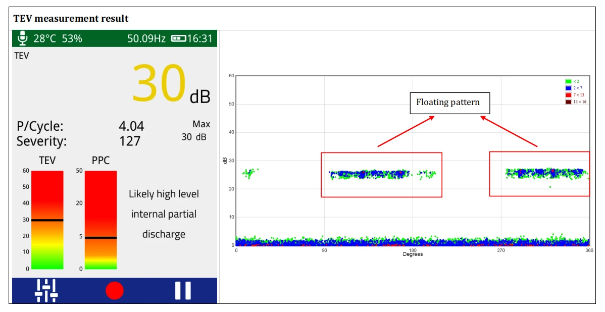
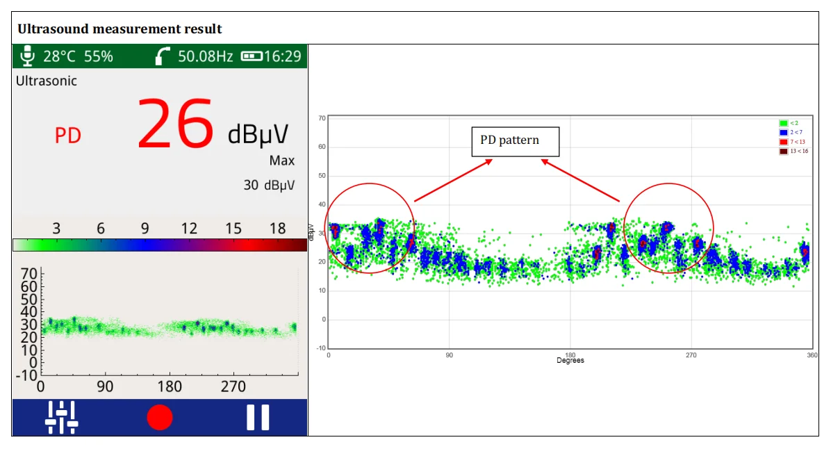
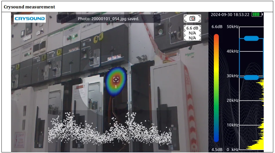
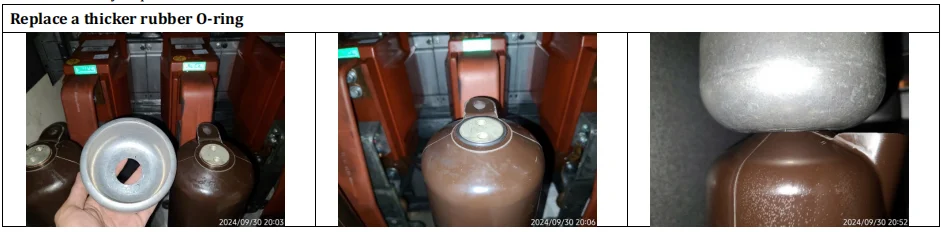
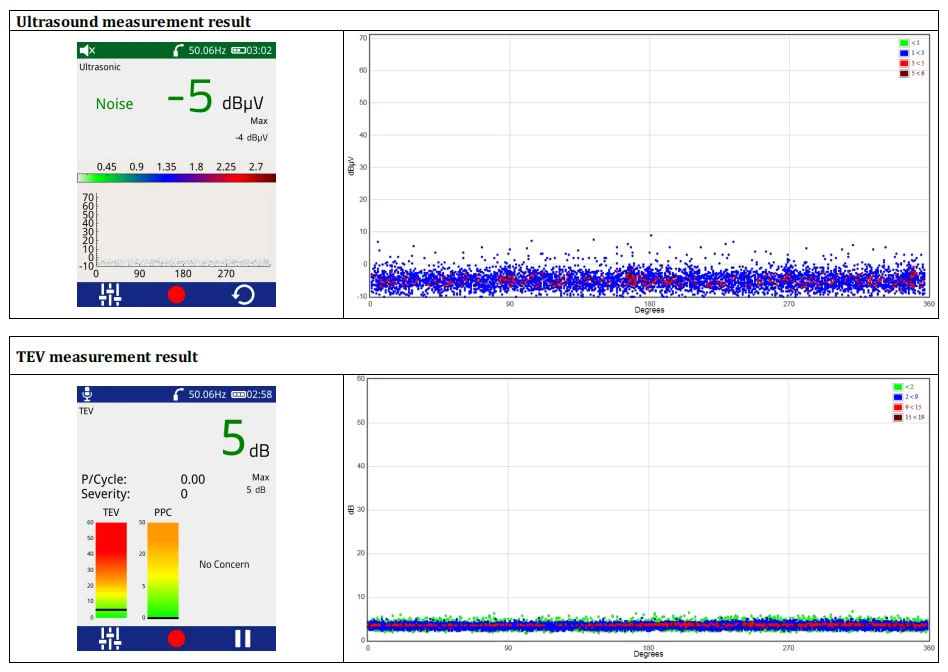
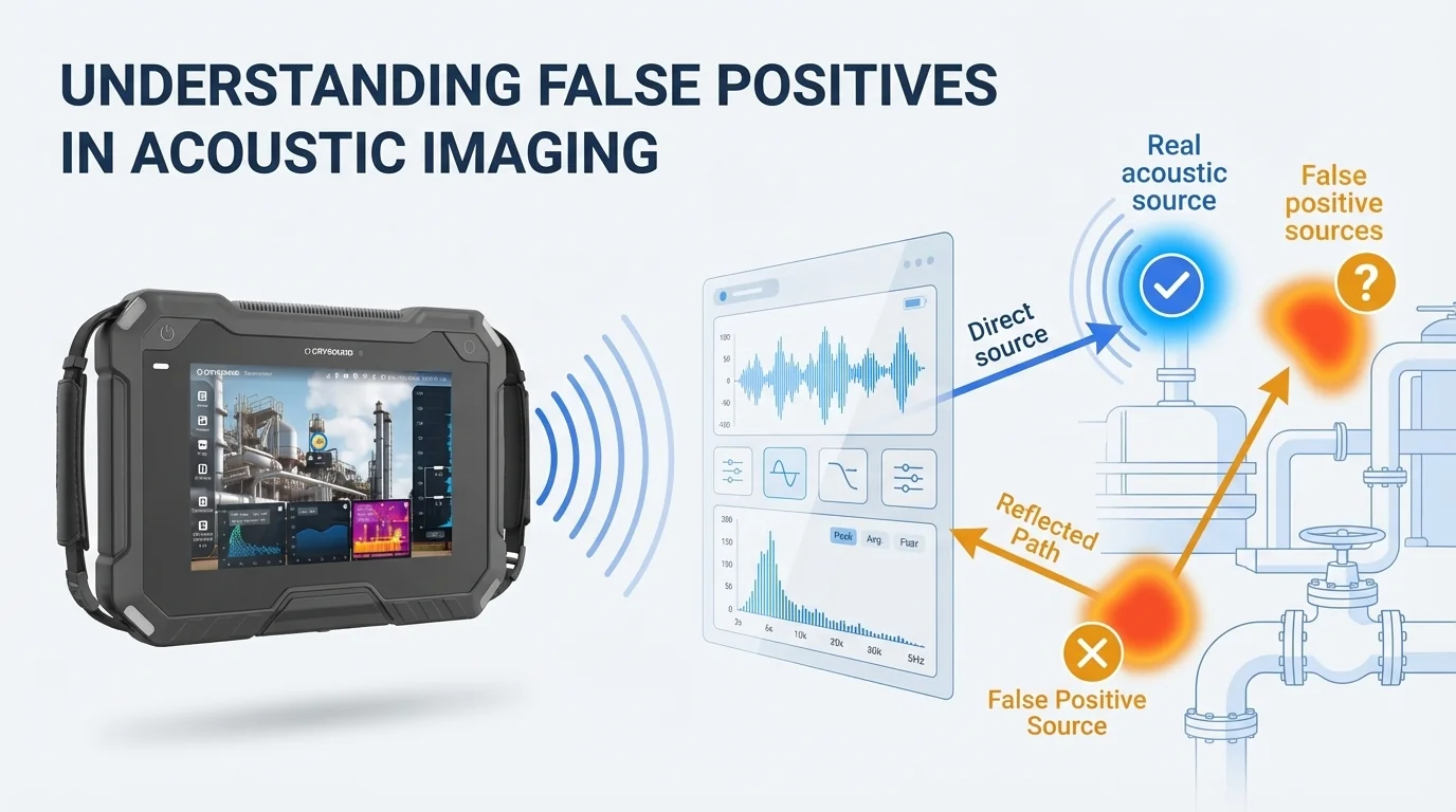
You're scanning overhead pipework in a compressor room when your acoustic camera shows a bright hotspot on a steel support beam. You walk over, listen carefully, and check the surface. Nothing. No hiss, no vibration, no leak. The image looks convincing, but the source is not actually on that beam. This is one of the most common acoustic imaging false positives engineers see in the field. Acoustic camera reflections, beamforming artifacts, and background noise can all create ghost images or false hotspots that look like real leaks, discharges, or mechanical faults. That does not mean the camera is malfunctioning. It means the operator needs to separate true sources from indirect paths and side responses. Based on field observations in reflective industrial environments, teams often find that 15–30% of initial acoustic indications should be treated as leads for verification rather than confirmed source locations. In this guide, we'll explain why an acoustic camera shows false hotspots, how to tell acoustic camera reflections from real leaks, and how to reduce beamforming artifacts in noisy factories without slowing down your inspection workflow. What Are False Positives in Acoustic Imaging? False positive (acoustic imaging): An apparent sound source indication on an acoustic camera display that does not correspond to an actual physical source at that location. Caused by physical phenomena including sound wave reflections, beamforming algorithm sidelobes, or environmental noise interference — not by equipment defect. Three related terms often get used interchangeably, but they describe different phenomena: False positive: Any indicated source that isn't real at the shown location Artifact: A systematic error pattern produced by the beamforming algorithm itself (e.g., sidelobes) Ghost image: A reflected or mirrored source — real sound arriving from an indirect path Understanding these distinctions matters because each type has different causes, different on-screen characteristics, and different solutions. Why Acoustic Cameras Show False Hotspots If your acoustic camera shows a hotspot on a wall, support beam, enclosure, or ceiling panel, the most common cause is a reflection rather than a leak at that exact surface. In other words, the hotspot may still be useful, but it is pointing to an indirect path instead of the true source location. If the display shows a halo, ring, or repeating spots around one strong source, that pattern is more likely a beamforming artifact than a second leak. And if the hotspot is broad, unstable, or spread across a noisy production area, environmental noise is usually a better explanation than a discrete defect. For teams using acoustic cameras in compressed air leak detection, it helps to pair this article with our acoustic camera guide and how acoustic imaging works explainer. If you need to quantify the cost of missed leaks before the next survey, use our air leak cost calculator. Common False Positives in Acoustic Cameras Reflections (Ghost Images) Sound waves bounce off hard, smooth surfaces — metal walls, concrete floors, glass panels, polished pipes — just like light reflects off a mirror. When your acoustic camera picks up both the direct sound and the reflected sound, the reflected path appears as a second source at a location where nothing is actually producing noise. Typical scenario: You're imaging a compressed air manifold mounted near a stainless steel wall. The display shows two hotspots — one on the manifold (real) and one on the wall behind it (ghost). The ghost image appears at roughly the same intensity and frequency as the real source. On-screen signature: Ghost images tend to appear at geometrically symmetrical positions relative to the reflecting surface. They share the same frequency spectrum as the real source and often appear at similar or slightly reduced intensity. Sidelobe Artifacts This is the most technically nuanced type. Beamforming algorithms work by mathematically "focusing" the microphone array on each point in the field of view. But just as a flashlight can't produce a perfectly sharp beam edge, beamforming produces a main lobe (the focused area) surrounded by sidelobes — weaker response regions that can register false sources. Typical scenario: You're imaging a single loud leak, but the display shows the main hotspot surrounded by a ring or pattern of secondary spots. These sidelobe artifacts are always clustered around the true source and become more pronounced when the source is loud relative to surrounding noise. On-screen signature: Sidelobes appear as a repeating pattern around the main source — often a ring, halo, or radial spoke pattern. Their intensity is always lower than the main lobe, and they maintain a fixed geometric relationship to the primary source regardless of scanning angle. Key factor: The number of microphone channels directly affects sidelobe levels. A 64-channel array produces more prominent sidelobes than a 128-channel array, which in turn produces more than a 200-channel array. Higher channel counts provide narrower main lobes and lower sidelobe floors. Advanced algorithms like CRYSOUND's HyperVision processing further suppress sidelobes beyond what standard delay-and-sum beamforming achieves. Environmental Noise Interference Not every unwanted indication is a reflection or algorithm artifact. Sometimes, your acoustic camera is accurately detecting a real sound — just not the one you're looking for. Background noise from HVAC systems, nearby machinery, overhead cranes, or even wind can register as apparent sources that get confused with your target. Typical scenario: During a compressed air leak survey in a manufacturing hall, you see multiple hotspots across a wide area. Some are genuine leaks. Others are background machinery noise that happens to fall within your selected frequency band. On-screen signature: Environmental noise sources typically have broader, more diffuse patterns than leaks (which appear as tight, focused hotspots). They also show different frequency characteristics — machinery noise tends to be narrower-band and harmonic, while leak noise is broadband and turbulent. Quick Comparison Type Cause On-Screen Signature Elimination Difficulty Reflections Sound bouncing off hard surfaces Symmetrical ghost image, same frequency as real source Moderate — multi-angle scan + frequency check Sidelobe artifacts Beamforming algorithm side response Ring/halo pattern around main source, lower intensity Low with advanced algorithms (HyperVision) Environmental noise Background machinery in frequency band Diffuse pattern, tonal/harmonic frequency profile Low — frequency filtering + Focus Function How to Identify False Positives: A 4-Step Process When you see an indication you're unsure about, run through these steps before logging it as a confirmed source: Angle change test. Move 2-3 meters to the side and re-scan the same area. Real sources stay in the same physical position on the image. Reflections shift or disappear as you change the angle of incidence. Sidelobes rotate with the main source. Frequency signature check. Switch to spectrum view (if your camera supports it) and examine the frequency profile. Compressed air leaks produce broadband, turbulent noise typically above 20 kHz. Machinery noise has distinct tonal peaks. If the "source" shares an identical spectrum with a known real source nearby, it's likely a reflection. Distance validation. If your camera allows distance-to-source measurement, check whether the indicated distance matches the physical geometry. A reflection off a wall 3 meters behind you will show a source distance that doesn't match the wall's position from your scanning location. Ultrasonic listening. Most acoustic cameras offer a downshift playback feature that converts the directionally-captured ultrasonic signal into audible sound through headphones. Point the camera at the suspect indication and listen. A real compressed air leak produces a distinctive broadband hiss. Sidelobe artifacts and reflections carry no independent acoustic signature — they sound identical to the main source. Environmental noise sounds tonal and harmonic. This lets you verify from your scanning position without walking to the indicated location. Techniques to Minimize False Positives 1. Select the Right Frequency Band Most acoustic cameras allow you to filter by frequency range. Narrowing the band to your target application reduces interference dramatically. For compressed air leaks, focus on 20–50 kHz. For partial discharge, 20–100 kHz. Excluding lower frequencies cuts out most machinery noise. 2. Use Advanced Beamforming Algorithms Not all beamforming is equal. Standard delay-and-sum (DAS) algorithms are computationally simple but produce higher sidelobe levels. Advanced algorithms apply spatial filtering to suppress sidelobes at the processing level. CRYSOUND's HyperVision algorithm, available on the CRY8124 and CRY8120 series, provides up to 10x processing power over standard beamforming, reducing sidelobe artifacts significantly without sacrificing real-time performance. 3. Adopt a Multi-Angle Scanning Protocol Make it standard practice to scan critical areas from at least two different positions. Compare the results. Sources that appear consistently in the same physical location are real. Sources that shift, disappear, or change intensity are false positives. This takes an extra 30 seconds per area and dramatically reduces misdiagnosis. Turning Artifacts into Allies: Using False Positives to Locate Sources Here's where experienced operators separate from beginners. False positives aren't just noise to eliminate — they carry information about the acoustic environment that you can exploit. Reflection Mapping If you see a ghost image on a metal wall, you've just learned something valuable: there's a real sound source at the geometrically mirrored position. The reflection tells you the sound wave's travel path. In complex piping environments where direct line-of-sight to a leak is blocked, reflected images on nearby surfaces can reveal the general direction and approximate distance of sources you can't see directly. Pro technique: When scanning in confined spaces with multiple reflective surfaces, intentionally note where ghost images appear. The pattern of reflections triangulates the true source location, even when the source is behind equipment or above a ceiling panel. Sidelobe Pattern Reading Sidelobes always radiate symmetrically from the main lobe. When you see a sidelobe pattern, the center of that pattern is your real source — guaranteed. In environments where obstructions partially block your view, the visible sidelobes can confirm the direction of a source that's partially hidden. If the sidelobe "ring" is only visible on one side, the true source is on the opposite side, behind whatever's blocking your view. Spatial Focusing (ROI Isolation) In noisy industrial environments, you can't shut down surrounding equipment just to get a cleaner acoustic image. Instead, use your camera's Focus Function: draw a region of interest (ROI) directly on the screen around the area you want to investigate. The camera restricts its beamforming analysis to that region only, effectively suppressing sound sources outside the selected area. This is particularly powerful when combined with frequency band filtering. Narrow the frequency range to your target application (e.g., 20–50 kHz for leak detection), then draw an ROI around the suspect zone. The double filter — spatial plus spectral — dramatically reduces environmental noise interference without requiring any change to the plant's operating conditions. What previously looked like a cluttered display with overlapping hotspots becomes a clean, focused view of the area that matters. Quick Reference Checklist Eliminating false positives: Set correct frequency band for target application Scan from at least two angles Check frequency spectrum of ambiguous sources Use ultrasonic listening to verify auditory signature before logging Leveraging false positives: Note reflection positions to triangulate hidden sources Read sidelobe patterns to confirm source direction Use Focus Function (ROI) to isolate target area from surrounding noise Need help diagnosing false positives? Talk to our application engineers → Frequently Asked Questions How common are false positives in acoustic imaging? Every acoustic camera produces some false positives. They are an inherent characteristic of beamforming physics, array geometry, and reflective environments rather than a product defect. With the right scanning workflow, most operators can tell a real source from a false hotspot within seconds. Why does my acoustic camera show a hotspot on the wall? The most common reason is reflection. The wall is acting like an acoustic mirror, so the camera detects indirect sound energy and maps it to the mirrored position. If the hotspot shifts or disappears when you change your scanning angle, you are likely looking at a reflection instead of a real source on that wall. What is the difference between a reflection and a beamforming artifact? A reflection is real sound reaching the array by an indirect path after bouncing off a surface. A beamforming artifact is a pattern generated by the imaging algorithm itself, often appearing as a halo or repeating side response around a strong source. Reflections usually move with geometry and angle; beamforming artifacts stay locked to the true source pattern. Can reflections be completely eliminated? No. As long as there are hard, smooth surfaces in the environment, sound will reflect. However, you can reduce their impact by scanning from multiple angles, matching spectra, and using region-of-interest controls to isolate the target area. Does a higher microphone channel count reduce artifacts? Yes. More channels generally provide a narrower main lobe and a lower sidelobe floor, which means fewer misleading side responses around strong sources. This is one reason acoustic camera specifications matter when you compare systems. How do I handle false positives in noisy factory environments? Use three filters together: narrow the frequency band to the target application, restrict the imaging area with an ROI or focus function, and confirm suspicious hotspots from a second angle. In most plants, that combination separates real leak-like sources from machinery noise fast enough for practical inspections. Can acoustic reflections actually help locate the real source? Yes. Reflections reveal the sound path, which means a ghost image can still tell you where to keep searching. In cluttered piping or enclosed machinery spaces, reflection patterns often help experienced operators triangulate the hidden source more quickly.