Octave-band analysis converts detailed spectra into standardized 1/1- and 1/3-octave bands using constant-percentage bandwidth on a logarithmic frequency axis. In this post, we explain the mathematical basis of CPB, why IEC 61260-1 and ANSI S1.11 define octave bands the way they do, and how band levels are computed in practice (FFT binning vs. filter-bank RMS). The goal: repeatable, comparable results for acoustics, NVH, and compliance measurements. What is octave-band analysis, and what problem does it solve? Octave-band analysis is a family of spectrum analysis methods that partition the frequency axis on a logarithmic scale into band-pass bands. Each band has a constant ratio between its upper and lower cut-off frequencies (constant percentage bandwidth, CPB). Within each band we ignore fine line-spectrum details and focus on total energy / RMS (or power) in that band. In other words, it is not “what happens at every 1 Hz,” but “how energy is distributed across equal relative bandwidths.” This representation naturally matches human hearing and many engineering systems, whose frequency resolution is often closer to a relative (log) scale than a fixed-Hz scale. It is a common reporting format required by many standards: room acoustics parameters, sound insulation ratings, environmental noise, machinery noise, wind/road noise, etc., often use 1/3-octave bands. From linear Hz to log frequency: why CPB looks more like an engineering language Using equal-width frequency bins (e.g., every 10 Hz) to accumulate energy leads to inconsistent behavior across the spectrum: At low frequencies, a 10 Hz bin may be too wide and can smear details. At high frequencies, a 10 Hz bin may be too narrow, giving higher variance and less stable estimates for random noise. In contrast, CPB bandwidth grows with frequency (Δf ∝ f). Each band covers a similar relative change, improving stability and repeatability—important for standardized testing. A visual intuition: bandwidth increases on a linear axis, but is uniform on a log axis Figure 1: the same 1/3-octave bands plotted on a linear frequency axis—bandwidth appears larger at high frequencies Each horizontal segment represents a 1/3-octave band [f1, f2]; the short vertical mark is the band center frequency fm. On a linear axis, higher-frequency bands look wider. Figure 2: the same bands on a logarithmic frequency axis—bands become evenly spaced (the essence of CPB) Once the horizontal axis is logarithmic, these bands appear equal-width/equal-spacing; this is exactly what “constant percentage bandwidth” means. These two figures capture the core idea: octave-band analysis uses equal steps on a log-frequency scale, not equal steps in Hz. Standards and terminology: what do IEC/ANSI/ISO systems actually specify? In practice, “doing 1/3-octave analysis” is constrained by more than just band edges. Standards specify (or strongly imply): how center frequencies are defined (exact vs nominal), the octave ratio definition (base-10 vs base-2), filter tolerances/classes, and even the measurement/averaging conventions used to form band levels. IEC 61260-1:2014 highlights: base-10 ratio, reference frequency, and center-frequency formulas IEC 61260-1:2014 is a key specification for octave-band and fractional-octave-band filters. It adopts a base-10 design: the octave frequency ratio is G = 10^(3/10) ≈ 1.99526 (very close to 2, but not exactly 2). The reference frequency is fr = 1000 Hz. It provides formulas for the exact mid-band (center) frequencies and specifies that the geometric mean of band-edge frequencies equals the center frequency. [1] Key formulas (rearranged from the standard): [1] If the fractional denominator b is odd (e.g., 1, 3, 5, ...): If b is even (e.g., 2, 4, 6, ...): And always: Why does the even-b case look “half-step shifted”? Intuitively, the center-frequency grid is evenly spaced on log(f). When b is even, IEC chooses a half-step offset relative to fr so that band edges align more neatly in common reporting conventions. In practice, a robust implementation is to generate the exact fm sequence using the standard’s formula, then compute edges via f1 = fm / G^(1/(2b)) and f2 = fm * G^(1/(2b)), and only then label bands by the usual nominal frequencies. View the data with OpenTest (IEC 61260-1 Octave-Band Analysis) -> Band edges, center frequency, and the bandwidth designator b Standards commonly use 1/b as the “bandwidth designator”: 1/1 is one octave, 1/3 is one-third octave, etc. [1] Once (G, b, fr) are chosen, the entire band set (centers and edges) is fixed mathematically. Exact vs nominal: why two “center frequencies” appear for the same band “Exact” center frequencies are used for mathematically consistent definitions and filter design; “nominal” values are used for labeling and reporting. [1] ISO 266:1997 defines preferred frequencies for acoustics measurements based on ISO 3 preferred-number series (R10), referenced to 1000 Hz. [2] As a result, the exact geometric sequence is typically labeled with familiar nominal values such as: 20, 25, 31.5, 40, 50, 63, 80, 100, 125, 160, …, 1k, 1.25k, 1.6k, 2k, 2.5k, 3.15k, …, 20k. Implementation tip: compute edges from exact frequencies; only round/display as nominal. This avoids drifting away from the standard. Base-10 vs base-2: why standards don’t insist on an exact 2:1 octave Although “octave” is often thought of as 2:1, IEC 61260-1 specifies base-10 (G=10^(3/10)) rather than G=2. Key motivations include: Alignment with decimal preferred-number series (ISO 266 is tied to R10). [2] International consistency: IEC 61260-1:2014 specifies base-10 and notes that base-2 designs are less likely to remain compliant far from the reference frequency. [1] In base-10, one-third octave corresponds to 10^(1/10) ≈ 1.258925 (also interpretable as 1/10 decade), which yields a clean mapping: 10 one-third-octave bands per decade. “10 one-third-octave bands = 1 decade”: why this matters With base-10 one-third-octave spacing, each step multiplies frequency by r = 10^(1/10). Therefore: 10 consecutive 1/3-octave bands multiply frequency by exactly 10 (one decade). This matches ISO 266/R10 conventions and simplifies tables, plotting, and communication. Standardization values readability and consistency as much as raw mathematical purity. Figure 3: Base-10 one-third-octave spacing—10 equal ratio steps per decade (×10 in frequency) ANSI S1.11 / ANSI/ASA S1.11: tolerance classes and a transient-signal caution ANSI S1.11 (and later ANSI/ASA adoptions aligned with IEC 61260-1) specify performance requirements for filter sets and analyzers, including tolerance classes (often class 0/1/2 depending on edition). [3][4] A practical caution in ANSI documents: for transient signals, different compliant implementations can produce different results. [3] This highlights that time response (group delay, ringing, averaging time constants) matters for transient analysis. What do class/mask/effective bandwidth actually control? “I used 1/3-octave bands” is not just about nominal band edges. Standards aim to ensure different instruments/algorithms yield comparable results by constraining: Frequency spacing: center-frequency sequence and edge definitions (base-10, exact/nominal, f1/f2). Magnitude response tolerance (mask): allowable ripple near passband and required attenuation away from center. Energy consistency for broadband noise: constraints on effective bandwidth so band levels are comparable across implementations. Effective bandwidth matters because real filters are not ideal brick walls. For broadband noise, the output energy depends on ∫|H(f)|^2 S(f)df. Differences in passband ripple, skirts, and roll-off can cause systematic offsets. Standards constrain effective bandwidth to keep such offsets within acceptable limits. [1][3][4] The transient caution is not a contradiction: masks mainly constrain steady-state frequency-domain behavior, while transients depend on phase/group delay, ringing, and time averaging. [3] Mathematics: band definitions, bandwidth, Q, and band indexing CPB and equal spacing on a log axis CPB is equivalent to equal-width spacing in log-frequency. If u = log(f), then every band spans a fixed Δu. Many spectra (e.g., 1/f-type) look smoother and statistically more stable in log frequency. Band-edge formulas from the geometric-mean definition (general 1/b form) IEC defines the center frequency as the geometric mean of the edges: fm = sqrt(f1 f2). [1] For 1/b octave bands, the edge ratio is typically f2/f1 = G^(1/b), where G is the octave ratio. Then: For base-10 one-third octave (b=3): G=10^(3/10). Adjacent center ratio is r = G^(1/3) = 10^(1/10) ≈ 1.258925; edge multiplier is k = 10^(1/20) ≈ 1.122018. Q-factor and resolution: octave analysis is constant-Q analysis Define Q = fm / (f2 − f1). For CPB bands, Δf = f2 − f1 scales with fm, so Q depends only on b and G (not on frequency). Quick reference (base-10, fr=1000 Hz): Fractional-octaveBand ratio f2/f1Relative bandwidth Δf/fmQ = fm/Δf1/11.9952620.7045921.4191/21.4125380.3471072.8811/31.2589250.2307684.3331/61.1220180.1151938.6811/121.0592540.05757317.369 Interpretation: for 1/3 octave, Q≈4.33 and each band is about 23% wide relative to its center. Finer bands (1/6, 1/12) give higher resolution but higher variance for random noise and typically require longer averaging. Band numbering (integer index) and formulaic enumeration Implementations often use an integer band index x. In IEC, x appears directly in the center-frequency formula: fm = fr * G^(x/b). [1] This provides a stable way to enumerate all bands covering a target frequency range and ensures contiguous, standard-consistent edges. For base-10: so and you can invert as Figure 4: Q factor for common fractional-octave bandwidths (base-10 definition) Two meanings of “1/3 octave”: base-2 vs base-10—do not mix them Some literature uses base-2: adjacent centers are 2^(1/3). IEC 61260-1 and much modern acoustics practice use base-10: adjacent centers are 10^(1/10). A quick check: if nominal centers look like 1.0k → 1.25k → 1.6k → 2.0k (R10 style), it is likely base-10. Mathematical definition of band levels: from PSD integration to dB reporting Continuous-frequency view: integrate PSD within the band Octave-band level is essentially the integral of power spectral density over a frequency band. For sound pressure p(t): For vibration (velocity/acceleration), the same logic applies with different units and reference quantities. Key point: because dB is logarithmic, any summation or averaging must be performed in the linear power/mean-square domain first. Two discrete implementations: filter-bank RMS vs FFT/PSD binning Filter-bank method: y_b(t)=BandPass_b{x(t)}, then compute mean(y_b^2) as band mean-square (optionally with time averaging). FFT/PSD binning method: estimate S_pp(f) (e.g., via periodogram/Welch), then numerically integrate/sum bins within [f1,f2]. For long, stationary signals, averaged results can be very close. For transients, sweeps, and short events, they often differ. Be explicit about what spectrum you have: magnitude, power, PSD (and dB/Hz) Magnitude spectrum |X(f)|: amplitude units (e.g., Pa), useful for tones/harmonics. Power spectrum |X(f)|²: mean-square units (Pa²). Power spectral density (PSD): mean-square per Hz (Pa²/Hz), most common for noise. Because octave-band levels represent band mean-square/power, you must end up integrating/summing in Pa² (or analogous) regardless of starting representation. Frequency resolution and one-sided spectra: Δf, 0..fs/2, and the “×2” rule FFT bin spacing is Δf = fs/N. A typical discrete approximation is: If you use a one-sided spectrum (0..fs/2), to conserve energy you typically multiply all non-DC and non-Nyquist bins by 2 (because negative-frequency power is folded into the positive side). Different software handles these conventions differently, so align definitions before comparing results. Window corrections: coherent gain (tones) vs ENBW (noise) are different Windowing reduces spectral leakage but changes scaling: For tone amplitude: correct by coherent gain (CG), often CG = sum(w)/N. For broadband noise/PSD: correct by equivalent noise bandwidth (ENBW), e.g., ENBW = fs·sum(w²)/(sum(w))². [9] CG controls peak amplitude; ENBW controls average noise-floor area. Octave-band levels are energy statistics and are more sensitive to ENBW. WindowCoherent Gain (CG)ENBW (bins)Rectangular1.0001.000Hann0.5001.500Hamming0.5401.363Blackman0.4201.727 Partial-bin weighting: what to do when band edges do not align to FFT bins Band edges rarely land exactly on bin frequencies. Treat PSD as approximately constant within each bin of width Δf, and weight boundary bins by their overlap fraction: This produces smoother, more physically consistent band levels when N or band edges change. Figure 5: Partial-bin weighting schematic when band edges do not align with FFT bins A unifying formula: both methods compute ∫|H_b(f)|² S_xx(f) df Both filter-bank and PSD binning can be written as: Brick-wall binning corresponds to |H_b|² being 1 inside [f1,f2] and 0 outside. A true standards-compliant filter has a roll-off and ripple, which is why standards constrain masks and effective bandwidth. Band aggregation: composing 1-octave from 1/3-octave, and forming total levels Under ideal partitioning and energy accounting: Three adjacent 1/3-octave bands can be combined to approximate one full octave band. Summing all band energies over a covered range yields the total energy. Always combine in the energy domain. If L_i are band levels in dB, energies are E_i = 10^(L_i/10). Then: IEC 61260-1 notes that fractional-octave results can be combined to form wider-band levels. [1] Effective bandwidth: why standards specify it Real filters are not ideal rectangles. For white noise (constant PSD S0), output mean-square is: For non-white spectra such as pink noise (PSD ~ 1/f), standards may define normalized effective bandwidth with weighting to maintain comparability across typical engineering noise spectra. [1] Practical implication: FFT “hard-binning” implicitly assumes a brick-wall filter with B_eff = (f2 − f1). A compliant octave filter has skirts, so B_eff can differ slightly (and by class). To match results, either approximate the standard’s |H(f)|² in the frequency domain or document the methodological difference. Why 1/3 octave is favored (math + perception + engineering trade-offs) Information density is “just right”: finer than 1 octave, steadier than very fine fractions A single octave band can be too coarse and hide spectral shape; very fine fractions (e.g., 1/12, 1/24) can be unstable and expensive: Higher estimator variance for random noise (each band captures less energy). More computation and higher reporting burden. Often more detail than regulations or rating schemes need. One-third octave is the classic compromise: enough resolution for engineering insight, stable enough for standardized measurements, and broadly supported by instruments and software. Psychoacoustics: critical bands in mid-frequencies are close to 1/3 octave Many psychoacoustics references describe ~24 critical bands across the audible range, and in the mid-frequency region the critical-bandwidth is often similar to a 1/3-octave bandwidth. [7][8] This makes 1/3 octave a natural intermediate representation for problems tied to perceived sound, while still being more standardized than Bark/ERB scales. Direct standards/application pull: many workflows mandate 1/3 octave I/O Once major standards define inputs/outputs in 1/3 octave, ecosystems (instruments, software, reporting templates) converge around it. Examples: Building acoustics ratings: ISO 717-1 references one-third-octave bands for single-number quantity calculations. [5] Room acoustics parameters (e.g., reverberation time) are commonly reported in octave/one-third-octave bands (ISO 3382 series). [6] Extra base-10 benefits: R10 tables, 10 bands/decade, readability 10 bands per decade: multiplying frequency by 10 corresponds to exactly 10 one-third-octave steps (very clean for log plots). R10 preferred numbers: 1.00, 1.25, 1.60, 2.00, 2.50, 3.15, 4.00, 5.00, 6.30, 8.00 (×10^n) are widely recognized and easy to communicate. Compared with base-2, decimal labeling is less awkward and cross-standard ambiguity is reduced. Octave-band analysis is typically implemented using either FFT binning or a filter bank. Keep reading -> Octave-Band Analysis Guide: FFT Binning vs. Filter Bank OpenTest integrates both methods. Download and get started now -> or fill out the form below ↓ to schedule a live demo. Explore more features and application stories at www.opentest.com. References [1] IEC 61260-1:2014 PDF sample (iTeh): https://cdn.standards.iteh.ai/samples/13383/3c4ae3e762b540cc8111744cb8f0ae8e/IEC-61260-1-2014.pdf [2] ISO 266:1997, Acoustics - Preferred frequencies (ISO): https://www.iso.org/obp/ui/ [3] ANSI S1.11-2004 preview PDF (ASA/ANSI): https://webstore.ansi.org/preview-pages/ASA/preview_ANSI%2BS1.11-2004.pdf [4] ANSI/ASA S1.11-2014/Part 1 / IEC 61260-1:2014 preview: https://webstore.ansi.org/preview-pages/ASA/preview_ANSI%2BASA%2BS1.11-2014%2BPart%2B1%2BIEC%2B61260-1-2014%2B%28R2019%29.pdf [5] ISO 717-1:2020 abstract (mentions one-third-octave usage): https://www.iso.org/standard/77435.html [6] ISO 3382-2:2008 abstract (room acoustics parameters): https://www.iso.org/standard/36201.html [7] Ansys Help: Bark scale and critical bands (mentions midrange close to third octave): https://ansyshelp.ansys.com/public/Views/Secured/corp/v252/en/Sound_SAS_UG/Sound/UG_SAS/bark_scale_and_critical_bands_179506.html [8] Simon Fraser University Sonic Studio Handbook: Critical Band and Critical Bandwidth: https://www.sfu.ca/sonic-studio-webdav/cmns/Handbook5/handbook/Critical_Band.html [9] MathWorks: ENBW definition example: https://www.mathworks.com/help/signal/ref/enbw.html

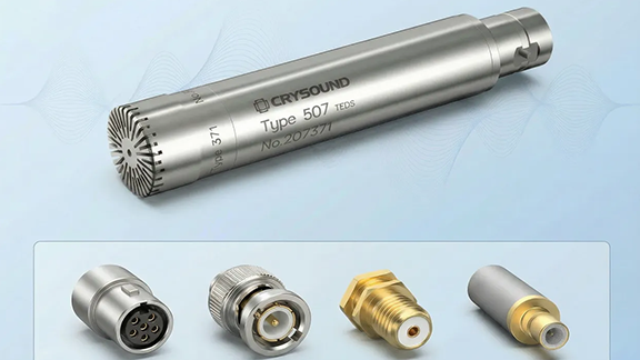
From the outside, a measurement microphone looks deceptively simple. But in real-world engineering, its interface options are surprisingly diverse: Lemo, BNC, Microdot, 10-32 UNF, M5, SMB… Many newcomers to acoustics ask questions like: Why can’t microphone interfaces be standardized? Why are cables often not interchangeable between microphones? What power and signal schemes are hidden behind different connectors? This article provides a structured overview of common measurement microphone interfaces, looking at physical connectors, powering methods, cable characteristics, and typical application-driven selection. Main Physical Interfaces for Measurement Microphones Below is a connector-by-connector summary, including the typical powering approach for each. Lemo (5-pin, 7-pin): The Classic Solution for Externally Polarized Microphones Lemo is a precision circular multi-pin connector and is the most common choice for externally polarized measurement microphones. The Lemo B series is widely used (e.g., 0B, 1B, 2B), and most standard measurement microphones adopt the Lemo 1B interface. Key Characteristics A multi-pin connector can carry multiple signals simultaneously, such as: Microphone output (analog signal) External polarization high voltage (typically 200 V) Preamplifier power supply Calibration/identification signals Additional benefits: Very reliable mechanical locking Well-suited for lab environments, metrology, and semi-anechoic chamber measurements where stability and traceability matter Notes on External Polarization Common polarization voltage is 200 V; some systems support switching between 0 V / 200 V Polarization voltage stability affects microphone sensitivity; in engineering practice, sensitivity variation is often treated as approximately proportional to voltage variation The preamplifier is typically powered separately (up to 120 V) but delivered via the same multi-pin connector Maximum output voltage can reach 50 Vp Includes pins for charge injection methods Separate output and ground paths help achieve lower noise In metrology labs, type testing, acoustic calibration, and high-precision semi-anechoic chamber work, the combination of “externally polarized microphone + Lemo multi-pin connector” is essentially a standard configuration. When not to use Lemo: Harsh environments with heavy contamination, oil exposure, and salt spray High costs of cables and connectors require careful trade-offs in field engineering applications BNC: The Most Common External Connector for IEPE Microphones Names like IEPE / ICP / CCP refer to the same general technology route: constant-current powering, where power and signal are transmitted on the same line (Constant Current Powering). In this system, the most common physical connector is the coaxial BNC. Interface and Powering Characteristics Coaxial structure, ideal for analog voltage transmission Bayonet lock (quick and reliable plug/unplug) Supports longer cable runs with good noise immunity Low cost and highly universal Typical IEPE Powering Parameters Constant current: 2–20 mA (common settings include 2 mA, 4 mA, 8 mA, etc.) Compliance voltage (supply capability): typically 18–24 V Maximum output voltage: generally around 8 Vp If the constant current is too low or the compliance voltage is insufficient, the maximum output signal swing is limited—directly affecting the maximum measurable SPL and the linear measurement range. In everyday testing such as engineering noise measurements, NVH, and environmental noise work, “IEPE microphone + BNC” has become the de facto standard. When not to use BNC: Applications requiring long-distance transmission of high-frequency signals, where signal attenuation becomes significant Applications involving frequent plugging and unplugging, to avoid an increased risk of poor electrical contact Microdot (10-32 UNF / M5): Lightweight Connectivity for Small Microphones Microdot is a threaded miniature coax connector widely used for small sensors (compact measurement microphones, accelerometers, etc.). It commonly uses a 10-32 UNF thread. What “10-32 UNF” Really Means This is simply an imperial fine-thread standard: Nominal diameter: 0.19 inch ≈ 4.826 mm Pitch: 1/32 inch ≈ 0.7938 mm Because 10-32 UNF is the typical thread used on Microdot connectors, the term “10-32 UNF” is often used informally to refer to the Microdot interface itself. What about M5? M5 is a metric thread standard: Nominal diameter: 5 mm Pitch: 0.8 mm Its dimensions are close to 10-32 UNF, and when tolerances are not extremely strict it can serve as a substitute—commonly seen in accelerometers or vibration microphones. Interface Characteristics Very compact; ideal for lightweight setups Threaded locking provides strong mechanical stability Commonly paired with IEPE powering Best for short runs and high-speed signal transmission When microphones must be placed in tight spaces, or where sensor mass/size is critical, Microdot is a common choice for compact, high-density installations. When not to use Microdot: Applications requiring quick connect/disconnect or frequent sensor replacement Use in systems with low constraints on installation space and requiring large-size connectors or high-power transmission, to avoid increased connection complexity and cost SMB (SubMiniature B): For High-Density Multi-Channel or Internal Connections SMB is a small “push-on” coaxial connector. Interface Characteristics Compact size supports high channel density Push-on structure enables fast connection Better high-frequency performance than BNC More suitable for semi-permanent internal wiring SMB is often best viewed as an engineering connector used inside equipment, rather than a field-plugging standard. When not to use Microdot: Applications involving frequent plugging and unplugging or repeated mechanical stress Use as a front-end connection interface for external devices, to avoid structural damage and reduced reliability Extended Interface Function: TEDS and Smart Identification In multi-channel and integrated systems, TEDS (Transducer Electronic Data Sheet) is increasingly common. By integrating a small memory chip into the sensor or cable, TEDS can store: Model and serial number Sensitivity Calibration date and other parameters Compatible front-end hardware or acquisition software can automatically read TEDS to: Identify the sensor type on each channel Load sensitivity and calibration coefficients automatically Reduce manual entry errors Save calibration time and labor At the connector level, TEDS is typically implemented by using certain pins in multi-pin Lemo connectors, or via overlay methods in specific BNC-based solutions. When planning an interface system, it’s wise to consider early on whether TEDS support is required. Why Are There So Many Interfaces? Connector diversity is best explained from three perspectives: Different Polarization and Powering Schemes Externally polarized microphones (≈ 200 V polarization) → better suited to multi-pin connectors like Lemo Prepolarized + IEPE systems → better suited to coaxial connectors like BNC / Microdot / SMB Different Scenarios and Priorities Laboratory / metrology: high stability, multiple signals in one cable, secure locking → Lemo Field engineering / environmental measurement: convenient wiring, strong universality → BNC + IEPE Miniaturization / high-density arrays: size and channel density first → Microdot / SMB Long Product Lifecycles and Backward Compatibility Measurement systems often have lifecycles of 10–20 years or more To avoid forcing users to replace large numbers of cables and front-end systems, manufacturers typically continue existing interface ecosystems Under long lifecycle constraints, “full unification” is often impractical and offers limited engineering return Typical Application Mapping (Quick Reference) Engineering noise, NVH, vibration/noise tests: BNC / MicrodotEasy wiring, many channels, low maintenance cost Precision lab measurement, type testing, metrology calibration: Lemo 7-pin / 5-pinSupports polarization HV and multiple signals; suitable for traceable high-precision measurement Acoustic arrays, multi-channel acquisition card systems: Microdot / SMBHigh channel density, compact wiring, easier system integration Long-term environmental noise monitoring systems: BNC / customized protected connectorsFocus on weather resistance, waterproofing, salt fog resistance, and stable long-distance transmission Conclusion The variety of measurement microphone interfaces is mainly the result of trade-offs between technology routes, application requirements, and historical compatibility—not simply a “lack of standards”. Taking NVH testing as an example: if an existing system uses BNC connectors to connect accelerometers, high-frequency signal attenuation and intermittent contact issues may occur in multi-channel array measurements. To improve connection reliability and signal quality, LEMO connectors with locking mechanisms and superior vibration resistance should be selected. After replacement, signal transmission stability is significantly improved, noise interference is reduced, and the consistency of test data is enhanced. You are welcome to learn more about microphone functions and hardware solutions on our website and use the “Get in touch” form to contact the CRYSOUND team.