Measure Sound Better
Blogs
In our previous blog post, "Abnormal Noise Detection: From Human Ears to AI"we discussed the key pain points of manual listening, introduced CRYSOUND's AI-based abnormal-noise testing solution, outlined the training approach at a high level, and showed how the system can be deployed on a TWS production line. In this post, we take the next step: we'll dive deeper into the analysis principles behind CRYSOUND's AI abnormal-noise algorithm, share practical test setups and real-world performance, and wrap up with a complete configuration checklist you can use to plan or validate your own deployment. Challenges Of Detecting Anomalies With Conventional Algorithms In real factories, true defects are both rare and highly diverse, which makes it difficult to collect a comprehensive library of abnormal sound patterns for supervised training. Even well-tuned—sometimes highly customized—rule-based algorithms rarely cover every abnormal signature. New defect modes, subtle variations, and shifting production conditions can fall outside predefined thresholds or feature templates, leading to missed detections (escapes). In the figure below, we compare two wav files that we generated manually. Figure 1: OK Wav Figure 2: NG Wav You can see that conventional checks—frequency response, THD, and a typical rub & buzz (R&B) algorithm—can hardly detect the injected low-level noise defect; the overall curve difference is only ~0.1 dB. In a simple FFT comparison, the two wav files do show some discrepancy, but in real production conditions the defect energy may be even lower, making it very likely to fall below fixed thresholds and slip through. By contrast, in the time–frequency representation , the abnormal signature is clearly visible, because it appears as a structured pattern over time rather than a small change in a single averaged curve. Figure 3: Analysis results Principle Of AI Abnormal Noise Algorithm CRYSOUND proposes an abnormal-noise detection approach built on a deep-learning framework that identifies defects by reconstructing the spectrogram and measuring what cannot be well reconstructed. This breaks through key limitations of traditional rule-based methods and, at the principle level, enables broader and more systematic defect coverage—especially for subtle, diverse, and previously unseen abnormal signatures. The figure below illustrates the core workflow behind our training and inference pipeline. Figure 4: Algorithm Flow Principle During model training, we build the algorithm following the workflow below. Figure 5: Algorithm Judgment Principle How To Use And Deploy The AI Algorithm Preparation First, prepare a Low-Noise Measurement Microphone / Low-noise Ear Simulator and a Microphone Power Supply to ensure you can capture subtle abnormal signatures while providing stable power to the mic. Figure 6: Low-Noise Measurement Microphone Next, you'll need a sound card to record the signal and upload the data to the host PC. Figure 7: Data Acquisition System Third, use a fixture or positioning jig to hold the product so that placement is repeatable and every recording is taken under consistent conditions. Finally, ensure a quiet and stable acoustic environment: in a lab, an anechoic chamber is ideal; on a production line, a sound-insulation box is typically used to control ambient noise and keep measurements consistent. Figure 8: Anechoic Room Figure 9: Anechoic Chamber Model Development First, create a test sequence in SonoLab, select "Deep Learning" and apply the setting. Next, select the appropriate AI abnormal-noise algorithm module and its corresponding API Figure 10: Sequence Interface 1 Then open Settings and specify the model type, as well as the file paths for the training dataset and test dataset. Click Train and wait for the model to finish training (Training time depends on your PC's hardware) Figure 11: Sequence Interface 2 During training, the status indicator turns yellow. Once training is complete, it switches to green and shows a "Training completed" message. Figure 12: Sequence Interface 3 Finally, place your test WAV files in the specified test folder and run the sequence. The model will start automatically and output the analysis results. Test Case Figure 13:Test Environment Figure 14:Test Curve System Block Diagram Figure 15: System Block Diagram 1 Figure 16: System Block Diagram 2 Equipment More technical details are available upon request—please use the "Get in touch" form below. Our team can share recommended settings and an on-site workflow tailored to your production conditions.
As A²B microphones and sensors are increasingly adopted in automotive applications, the demand for reliable testing in both R&D and production is also growing. This article explains why A²B testing matters, highlights the advantages of A²B over traditional analog cabling in terms of interconnect and scalability, outlines key measurement KPIs (such as frequency response, THD+N, phase/polarity, and SNR), and presents a typical test-bench setup along with the corresponding solution configuration. Why A²B Microphone and Sensor Testing Matters In-cabin audio is no longer just "music playback". Modern vehicles depend on high-performance acoustic sensing for hands-free calling, in-cabin communication, voice assistants, ANC/RNC, and more—and these features increasingly rely on multiple microphones and even accelerometers deployed around the cabin. ADI notes that the rapid expansion of audio-, voice-, and acoustics-related applications is a key trend, and that new digital microphone and connectivity approaches are enabling broader adoption. To deliver consistent performance, teams need a test workflow that is repeatable across different node positions, harness lengths, and configurations—without turning every debug session into a custom project. The Interconnect Shift: From Shielded Analog Cables to Digital A²B Historically, scaling microphone counts often meant scaling shielded analog cabling, which adds weight, cost, and integration burden—sometimes limiting these features to premium vehicle segments. A²B (Automotive Audio Bus) addresses that interconnect problem by enabling a scalable, networked digital audio architecture with deterministic behavior—exactly what timing-sensitive acoustic applications need. Figures a and b show how such a design may be realized with the traditional analog and the digital A²B systems, respectively. Figure 1 (a) Analog system design with analog mic elements (shielded wires). (b) Digital system design with digital mic elements (A²B technology and UTP wires). What You'll Measure: Key A²B Microphone KPIs Frequency Response (FR) THD+N Phase / polarity (and channel-to-channel consistency for arrays) SNR AOP (if required by your program/spec) Typical Block Diagram-What the Bench Looks Like At CRYSOUND, we provide more than just the CRY580 A²B interface. We offer a full automotive audio testing solution, including audio acquisition cards, microphones and sensors, acoustic sources, custom fixtures, acoustic test boxes, and vibration shakers, delivering a complete and streamlined testing experience. Figure 2 Here's a description of the testing block diagram, including the use of the latest OpenTest Audio Test & Measurement Software https://opentest.com Solution BOM List The value of end-to-end delivery: reducing system integration time and minimizing coordination costs between multiple suppliers. We cover everything from R&D to production line testing. Figure 3 BOM list of the solution If you'd like to learn more about A²B testing, please fill out the Get in touch form below and we'll reach out shoutly.