December 23, 2025
Octave-Band Analysis: The Mathematical and Engineering Rationale
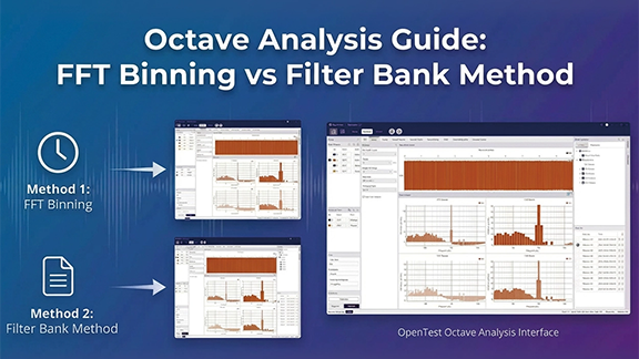
Octave-band analysis converts detailed spectra into standardized 1/1- and 1/3-octave bands using constant-percentage bandwidth on a logarithmic frequency axis. In this post, we explain the mathematical basis of CPB, why IEC 61260-1 and ANSI S1.11 define octave bands the way they do, and how band levels are computed in practice (FFT binning vs. filter-bank RMS). The goal: repeatable, comparable results for acoustics, NVH, and compliance measurements.
What is octave-band analysis, and what problem does it solve?
Octave-band analysis is a family of spectrum analysis methods that partition the frequency axis on a logarithmic scale into band-pass bands. Each band has a constant ratio between its upper and lower cut-off frequencies (constant percentage bandwidth, CPB). Within each band we ignore fine line-spectrum details and focus on total energy / RMS (or power) in that band.
In other words, it is not “what happens at every 1 Hz,” but “how energy is distributed across equal relative bandwidths.”
This representation naturally matches human hearing and many engineering systems, whose frequency resolution is often closer to a relative (log) scale than a fixed-Hz scale.
- It is a common reporting format required by many standards: room acoustics parameters, sound insulation ratings, environmental noise, machinery noise, wind/road noise, etc., often use 1/3-octave bands.
From linear Hz to log frequency: why CPB looks more like an engineering language
Using equal-width frequency bins (e.g., every 10 Hz) to accumulate energy leads to inconsistent behavior across the spectrum:
- At low frequencies, a 10 Hz bin may be too wide and can smear details.
- At high frequencies, a 10 Hz bin may be too narrow, giving higher variance and less stable estimates for random noise.
In contrast, CPB bandwidth grows with frequency (Δf ∝ f). Each band covers a similar relative change, improving stability and repeatability—important for standardized testing.
A visual intuition: bandwidth increases on a linear axis, but is uniform on a log axis

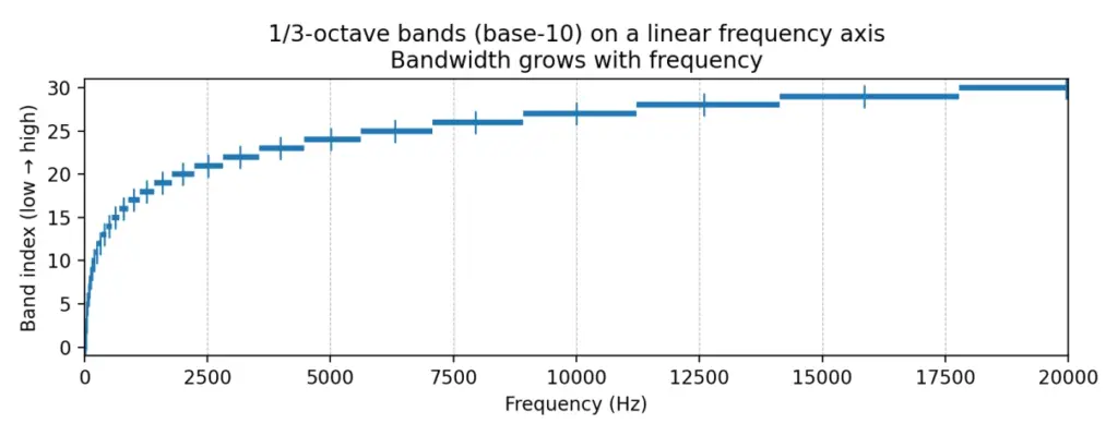
Figure 1: the same 1/3-octave bands plotted on a linear frequency axis—bandwidth appears larger at high frequencies
Each horizontal segment represents a 1/3-octave band [f1, f2]; the short vertical mark is the band center frequency fm. On a linear axis, higher-frequency bands look wider.

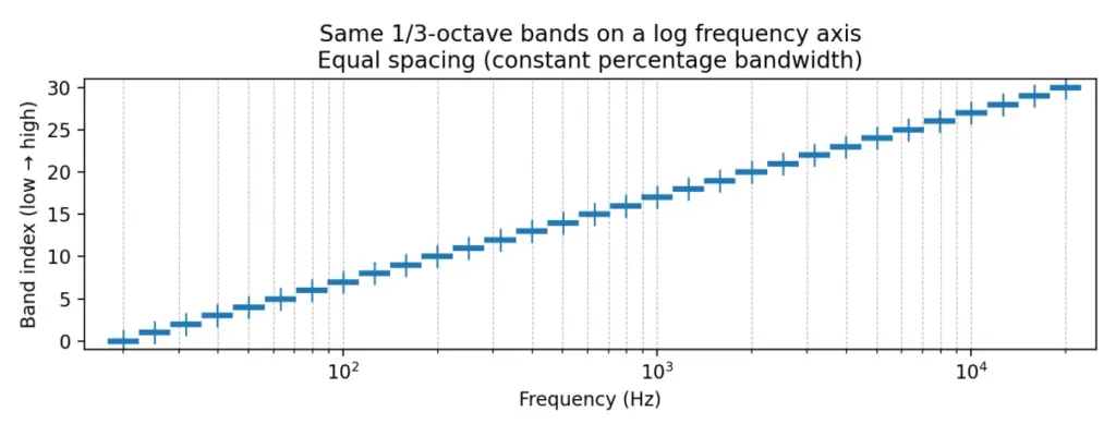
Figure 2: the same bands on a logarithmic frequency axis—bands become evenly spaced (the essence of CPB)
Once the horizontal axis is logarithmic, these bands appear equal-width/equal-spacing; this is exactly what “constant percentage bandwidth” means.
These two figures capture the core idea: octave-band analysis uses equal steps on a log-frequency scale, not equal steps in Hz.
Standards and terminology: what do IEC/ANSI/ISO systems actually specify?
In practice, “doing 1/3-octave analysis” is constrained by more than just band edges. Standards specify (or strongly imply): how center frequencies are defined (exact vs nominal), the octave ratio definition (base-10 vs base-2), filter tolerances/classes, and even the measurement/averaging conventions used to form band levels.
IEC 61260-1:2014 highlights: base-10 ratio, reference frequency, and center-frequency formulas
IEC 61260-1:2014 is a key specification for octave-band and fractional-octave-band filters. It adopts a base-10 design: the octave frequency ratio is G = 10^(3/10) ≈ 1.99526 (very close to 2, but not exactly 2). The reference frequency is fr = 1000 Hz. It provides formulas for the exact mid-band (center) frequencies and specifies that the geometric mean of band-edge frequencies equals the center frequency. [1]
Key formulas (rearranged from the standard): [1]

If the fractional denominator b is odd (e.g., 1, 3, 5, …):

If b is even (e.g., 2, 4, 6, …):

And always:

Why does the even-b case look “half-step shifted”? Intuitively, the center-frequency grid is evenly spaced on log(f). When b is even, IEC chooses a half-step offset relative to fr so that band edges align more neatly in common reporting conventions. In practice, a robust implementation is to generate the exact fm sequence using the standard’s formula, then compute edges via f1 = fm / G^(1/(2b)) and f2 = fm * G^(1/(2b)), and only then label bands by the usual nominal frequencies.
View the data with OpenTest (IEC 61260-1 Octave-Band Analysis) ->
Band edges, center frequency, and the bandwidth designator b
Standards commonly use 1/b as the “bandwidth designator”: 1/1 is one octave, 1/3 is one-third octave, etc. [1] Once (G, b, fr) are chosen, the entire band set (centers and edges) is fixed mathematically.
Exact vs nominal: why two “center frequencies” appear for the same band
“Exact” center frequencies are used for mathematically consistent definitions and filter design; “nominal” values are used for labeling and reporting. [1] ISO 266:1997 defines preferred frequencies for acoustics measurements based on ISO 3 preferred-number series (R10), referenced to 1000 Hz. [2]
As a result, the exact geometric sequence is typically labeled with familiar nominal values such as:
20, 25, 31.5, 40, 50, 63, 80, 100, 125, 160, …, 1k, 1.25k, 1.6k, 2k, 2.5k, 3.15k, …, 20k.
Implementation tip: compute edges from exact frequencies; only round/display as nominal. This avoids drifting away from the standard.
Base-10 vs base-2: why standards don’t insist on an exact 2:1 octave
Although “octave” is often thought of as 2:1, IEC 61260-1 specifies base-10 (G=10^(3/10)) rather than G=2. Key motivations include:
- Alignment with decimal preferred-number series (ISO 266 is tied to R10). [2]
- International consistency: IEC 61260-1:2014 specifies base-10 and notes that base-2 designs are less likely to remain compliant far from the reference frequency. [1]
In base-10, one-third octave corresponds to 10^(1/10) ≈ 1.258925 (also interpretable as 1/10 decade), which yields a clean mapping: 10 one-third-octave bands per decade.
“10 one-third-octave bands = 1 decade”: why this matters
With base-10 one-third-octave spacing, each step multiplies frequency by r = 10^(1/10). Therefore:
- 10 consecutive 1/3-octave bands multiply frequency by exactly 10 (one decade).
- This matches ISO 266/R10 conventions and simplifies tables, plotting, and communication.
- Standardization values readability and consistency as much as raw mathematical purity.

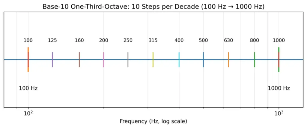
Figure 3: Base-10 one-third-octave spacing—10 equal ratio steps per decade (×10 in frequency)
ANSI S1.11 / ANSI/ASA S1.11: tolerance classes and a transient-signal caution
ANSI S1.11 (and later ANSI/ASA adoptions aligned with IEC 61260-1) specify performance requirements for filter sets and analyzers, including tolerance classes (often class 0/1/2 depending on edition). [3][4]
A practical caution in ANSI documents: for transient signals, different compliant implementations can produce different results. [3] This highlights that time response (group delay, ringing, averaging time constants) matters for transient analysis.
What do class/mask/effective bandwidth actually control?
“I used 1/3-octave bands” is not just about nominal band edges. Standards aim to ensure different instruments/algorithms yield comparable results by constraining:
- Frequency spacing: center-frequency sequence and edge definitions (base-10, exact/nominal, f1/f2).
- Magnitude response tolerance (mask): allowable ripple near passband and required attenuation away from center.
- Energy consistency for broadband noise: constraints on effective bandwidth so band levels are comparable across implementations.
Effective bandwidth matters because real filters are not ideal brick walls. For broadband noise, the output energy depends on ∫|H(f)|^2 S(f)df. Differences in passband ripple, skirts, and roll-off can cause systematic offsets. Standards constrain effective bandwidth to keep such offsets within acceptable limits. [1][3][4]
The transient caution is not a contradiction: masks mainly constrain steady-state frequency-domain behavior, while transients depend on phase/group delay, ringing, and time averaging. [3]
Mathematics: band definitions, bandwidth, Q, and band indexing
CPB and equal spacing on a log axis
CPB is equivalent to equal-width spacing in log-frequency. If u = log(f), then every band spans a fixed Δu. Many spectra (e.g., 1/f-type) look smoother and statistically more stable in log frequency.
Band-edge formulas from the geometric-mean definition (general 1/b form)
IEC defines the center frequency as the geometric mean of the edges: fm = sqrt(f1 f2). [1] For 1/b octave bands, the edge ratio is typically f2/f1 = G^(1/b), where G is the octave ratio. Then:


For base-10 one-third octave (b=3): G=10^(3/10). Adjacent center ratio is r = G^(1/3) = 10^(1/10) ≈ 1.258925; edge multiplier is k = 10^(1/20) ≈ 1.122018.
Q-factor and resolution: octave analysis is constant-Q analysis
Define Q = fm / (f2 − f1). For CPB bands, Δf = f2 − f1 scales with fm, so Q depends only on b and G (not on frequency).


Quick reference (base-10, fr=1000 Hz):
| Fractional-octave | Band ratio f2/f1 | Relative bandwidth Δf/fm | Q = fm/Δf |
| 1/1 | 1.995262 | 0.704592 | 1.419 |
| 1/2 | 1.412538 | 0.347107 | 2.881 |
| 1/3 | 1.258925 | 0.230768 | 4.333 |
| 1/6 | 1.122018 | 0.115193 | 8.681 |
| 1/12 | 1.059254 | 0.057573 | 17.369 |
Interpretation: for 1/3 octave, Q≈4.33 and each band is about 23% wide relative to its center. Finer bands (1/6, 1/12) give higher resolution but higher variance for random noise and typically require longer averaging.
Band numbering (integer index) and formulaic enumeration
Implementations often use an integer band index x. In IEC, x appears directly in the center-frequency formula: fm = fr * G^(x/b). [1] This provides a stable way to enumerate all bands covering a target frequency range and ensures contiguous, standard-consistent edges.
For base-10:

so

and you can invert as


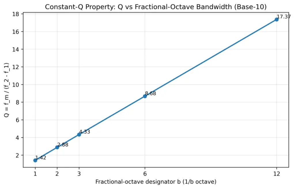
Figure 4: Q factor for common fractional-octave bandwidths (base-10 definition)
Two meanings of “1/3 octave”: base-2 vs base-10—do not mix them
Some literature uses base-2: adjacent centers are 2^(1/3). IEC 61260-1 and much modern acoustics practice use base-10: adjacent centers are 10^(1/10). A quick check: if nominal centers look like 1.0k → 1.25k → 1.6k → 2.0k (R10 style), it is likely base-10.
Mathematical definition of band levels: from PSD integration to dB reporting
Continuous-frequency view: integrate PSD within the band
Octave-band level is essentially the integral of power spectral density over a frequency band. For sound pressure p(t):


For vibration (velocity/acceleration), the same logic applies with different units and reference quantities.
Key point: because dB is logarithmic, any summation or averaging must be performed in the linear power/mean-square domain first.
Two discrete implementations: filter-bank RMS vs FFT/PSD binning
Filter-bank method: y_b(t)=BandPass_b{x(t)}, then compute mean(y_b^2) as band mean-square (optionally with time averaging).
FFT/PSD binning method: estimate S_pp(f) (e.g., via periodogram/Welch), then numerically integrate/sum bins within [f1,f2].
For long, stationary signals, averaged results can be very close. For transients, sweeps, and short events, they often differ.
Be explicit about what spectrum you have: magnitude, power, PSD (and dB/Hz)
- Magnitude spectrum |X(f)|: amplitude units (e.g., Pa), useful for tones/harmonics.
- Power spectrum |X(f)|²: mean-square units (Pa²).
- Power spectral density (PSD): mean-square per Hz (Pa²/Hz), most common for noise.
Because octave-band levels represent band mean-square/power, you must end up integrating/summing in Pa² (or analogous) regardless of starting representation.
Frequency resolution and one-sided spectra: Δf, 0..fs/2, and the “×2” rule
FFT bin spacing is Δf = fs/N. A typical discrete approximation is:

If you use a one-sided spectrum (0..fs/2), to conserve energy you typically multiply all non-DC and non-Nyquist bins by 2 (because negative-frequency power is folded into the positive side). Different software handles these conventions differently, so align definitions before comparing results.
Window corrections: coherent gain (tones) vs ENBW (noise) are different
Windowing reduces spectral leakage but changes scaling:
- For tone amplitude: correct by coherent gain (CG), often CG = sum(w)/N.
- For broadband noise/PSD: correct by equivalent noise bandwidth (ENBW), e.g., ENBW = fs·sum(w²)/(sum(w))². [9]
CG controls peak amplitude; ENBW controls average noise-floor area. Octave-band levels are energy statistics and are more sensitive to ENBW.
| Window | Coherent Gain (CG) | ENBW (bins) |
| Rectangular | 1.000 | 1.000 |
| Hann | 0.500 | 1.500 |
| Hamming | 0.540 | 1.363 |
| Blackman | 0.420 | 1.727 |
Partial-bin weighting: what to do when band edges do not align to FFT bins
Band edges rarely land exactly on bin frequencies. Treat PSD as approximately constant within each bin of width Δf, and weight boundary bins by their overlap fraction:


This produces smoother, more physically consistent band levels when N or band edges change.

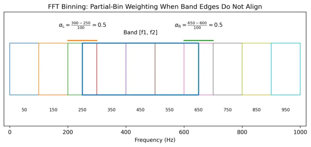
Figure 5: Partial-bin weighting schematic when band edges do not align with FFT bins
A unifying formula: both methods compute ∫|H_b(f)|² S_xx(f) df
Both filter-bank and PSD binning can be written as:

Brick-wall binning corresponds to |H_b|² being 1 inside [f1,f2] and 0 outside. A true standards-compliant filter has a roll-off and ripple, which is why standards constrain masks and effective bandwidth.
Band aggregation: composing 1-octave from 1/3-octave, and forming total levels
Under ideal partitioning and energy accounting:
- Three adjacent 1/3-octave bands can be combined to approximate one full octave band.
- Summing all band energies over a covered range yields the total energy.
Always combine in the energy domain.
If L_i are band levels in dB, energies are E_i = 10^(L_i/10). Then:

IEC 61260-1 notes that fractional-octave results can be combined to form wider-band levels. [1]
Effective bandwidth: why standards specify it
Real filters are not ideal rectangles. For white noise (constant PSD S0), output mean-square is:


For non-white spectra such as pink noise (PSD ~ 1/f), standards may define normalized effective bandwidth with weighting to maintain comparability across typical engineering noise spectra. [1]
Practical implication: FFT “hard-binning” implicitly assumes a brick-wall filter with B_eff = (f2 − f1). A compliant octave filter has skirts, so B_eff can differ slightly (and by class). To match results, either approximate the standard’s |H(f)|² in the frequency domain or document the methodological difference.
Why 1/3 octave is favored (math + perception + engineering trade-offs)
Information density is “just right”: finer than 1 octave, steadier than very fine fractions
A single octave band can be too coarse and hide spectral shape; very fine fractions (e.g., 1/12, 1/24) can be unstable and expensive:
- Higher estimator variance for random noise (each band captures less energy).
- More computation and higher reporting burden.
- Often more detail than regulations or rating schemes need.
One-third octave is the classic compromise: enough resolution for engineering insight, stable enough for standardized measurements, and broadly supported by instruments and software.
Psychoacoustics: critical bands in mid-frequencies are close to 1/3 octave
Many psychoacoustics references describe ~24 critical bands across the audible range, and in the mid-frequency region the critical-bandwidth is often similar to a 1/3-octave bandwidth. [7][8] This makes 1/3 octave a natural intermediate representation for problems tied to perceived sound, while still being more standardized than Bark/ERB scales.
Direct standards/application pull: many workflows mandate 1/3 octave I/O
Once major standards define inputs/outputs in 1/3 octave, ecosystems (instruments, software, reporting templates) converge around it. Examples:
- Building acoustics ratings: ISO 717-1 references one-third-octave bands for single-number quantity calculations. [5]
- Room acoustics parameters (e.g., reverberation time) are commonly reported in octave/one-third-octave bands (ISO 3382 series). [6]
Extra base-10 benefits: R10 tables, 10 bands/decade, readability
- 10 bands per decade: multiplying frequency by 10 corresponds to exactly 10 one-third-octave steps (very clean for log plots).
- R10 preferred numbers: 1.00, 1.25, 1.60, 2.00, 2.50, 3.15, 4.00, 5.00, 6.30, 8.00 (×10^n) are widely recognized and easy to communicate.
- Compared with base-2, decimal labeling is less awkward and cross-standard ambiguity is reduced.
Octave-band analysis is typically implemented using either FFT binning or a filter bank. Keep reading -> Octave-Band Analysis Guide: FFT Binning vs. Filter Bank
OpenTest integrates both methods. Download and get started now -> or fill out the form below ↓ to schedule a live demo.
Explore more features and application stories at www.opentest.com.
References
[1] IEC 61260-1:2014 PDF sample (iTeh): https://cdn.standards.iteh.ai/samples/13383/3c4ae3e762b540cc8111744cb8f0ae8e/IEC-61260-1-2014.pdf
[2] ISO 266:1997, Acoustics – Preferred frequencies (ISO): https://www.iso.org/obp/ui/
[3] ANSI S1.11-2004 preview PDF (ASA/ANSI): https://webstore.ansi.org/preview-pages/ASA/preview_ANSI%2BS1.11-2004.pdf
[4] ANSI/ASA S1.11-2014/Part 1 / IEC 61260-1:2014 preview: https://webstore.ansi.org/preview-pages/ASA/preview_ANSI%2BASA%2BS1.11-2014%2BPart%2B1%2BIEC%2B61260-1-2014%2B%28R2019%29.pdf
[5] ISO 717-1:2020 abstract (mentions one-third-octave usage): https://www.iso.org/standard/77435.html
[6] ISO 3382-2:2008 abstract (room acoustics parameters): https://www.iso.org/standard/36201.html
[7] Ansys Help: Bark scale and critical bands (mentions midrange close to third octave): https://ansyshelp.ansys.com/public/Views/Secured/corp/v252/en/Sound_SAS_UG/Sound/UG_SAS/bark_scale_and_critical_bands_179506.html
[8] Simon Fraser University Sonic Studio Handbook: Critical Band and Critical Bandwidth: https://www.sfu.ca/sonic-studio-webdav/cmns/Handbook5/handbook/Critical_Band.html
[9] MathWorks: ENBW definition example: https://www.mathworks.com/help/signal/ref/enbw.html
Related Products
Get in touch
Read more
Connect Multiple DAQs and Audio Interfaces in OpenTest
In industrial testing, research, and quality validation, data acquisition devices (DAQs / audio interfaces / measurement microphone front-ends) are the “front door” of the entire system. As technology and applications become more specialized, a wide variety of DAQ devices has emerged:
- High-precision front-ends designed specifically for acoustics and vibration
- General-purpose dynamic signal acquisition modules
- Common USB sound cards and measurement microphones
Hardware is not the bottleneck anymore. The real challenge is:
How do you connect, configure, and manage devices from different brands and protocols in one software platform?
OpenTest is built around this pain point. With an open, multi-protocol hardware access architecture, it turns acquisition from “isolated devices” into a unified platform, enabling cross-brand, multi-device data acquisition and analysis.

Multi-Protocol Hardware Access: Reducing Vendor Lock-In
OpenTest supports several mainstream connection methods. You can choose the appropriate protocol based on your hardware type and driver environment (actual compatibility depends on software version and device drivers):
- openDAQ – For open DAQ integration. Used to connect open hardware such as CRYSOUND SonoDAQ and manage channels and acquisition parameters in a unified way
- ASIO / WASAPI / MME / Core Audio – Mainstream audio interfaces on Windows and macOS, supporting professional audio interfaces and USB measurement microphones such as RME, Echo, miniDSP, etc.
- Other proprietary protocols – Can be added according to project requirements

This means you no longer need to be locked into a single hardware brand or a single piece of software. Existing devices can be brought smoothly under one platform for centralized management.
Multi-Device Collaboration: One Project, Many Acquisition Tasks
Complex tests often require multiple signal sources to be acquired together, for example:
- Dynamic signals such as microphones and accelerometers
- Operating parameters such as speed, temperature, pressure, torque
- Auxiliary audio paths for monitoring and playback
With OpenTest’s multi-protocol architecture, you can manage multiple devices within the same project. For NVH and structural testing, this kind of cross-device collaboration significantly reduces repetitive work like:
Recording in multiple software tools → exporting → manual time alignment → re-analysis
Getting Started: Connecting Devices Quickly
- Connect your data acquisition device to the PC running OpenTest
- USB connection, or
- Network connection (ensure the device and PC are on the same subnet)
- In the Hardware Setup panel, click the “+” icon in the upper-right corner. OpenTest will automatically scan for connected devices
- Check the devices you want to use and click Confirm to add them to the active device list
- Switch to the Channel Setup list, click the “+” icon in the upper-right corner, select the channels required for the current project (channels from different devices can be combined), and click Confirm to add them to the project
- Select the channels; OpenTest will automatically start real-time monitoring and analysis. You can then switch to different measurement modules according to your test needs

Presets + Fine Tuning: Easy to Start, Easy to Standardize
To help teams enter the testing state quickly, OpenTest supports a “presets + adjustments” configuration approach:
- Turn commonly used hardware parameters and acquisition settings into reusable templates
- Apply templates directly when creating a new project to avoid starting from scratch
- Still keep full flexibility to fine-tune settings for different operating conditions and devices
For production line or regression testing, templating adds an important benefit: uniform test conditions, comparable results, and traceable processes across time and across operators.
Logging and Monitoring: Designed for Long-Term Stability
For long-duration, multi-device acquisition, the worst case is discovering that something dropped out halfway. OpenTest provides observability features to address this:
- Device and channel status monitoring – Quickly detect disconnections, overloads, and abnormal inputs
- Operation and error logs – Record key actions and error events to support troubleshooting and process optimization
This is especially critical for continuous production testing and durability tests, significantly reducing the chance of “realizing halfway through that nothing was actually recorded.”
Typical Application Scenarios
- Acoustics and vibration R&D – Use the same platform to connect front-end DAQs and audio interfaces, quickly complete acquisition, analysis, and report generation
- Automotive NVH / structural testing – Acquire noise, vibration, and operating parameters together, minimizing cross-software alignment work
- Production line automated testing – Template-based configuration + monitoring/logging + automated reporting to improve consistency and traceability
OpenTest’s goal is not to make you replace all your hardware, but to bring your existing hardware together on one platform so that data acquisition becomes more efficient, more controllable, and much easier to standardize.
Visit www.opentest.com to learn more about OpenTest features and hardware options, or contact the CRYSOUND team for demos and application support.
Octave-Band Analysis Guide: FFT Binning vs. Filter Bank Method
Octave-band analysis can be implemented in two fundamentally different ways: FFT binning (integrating PSD/FFT bins into 1/1- and 1/3-octave bands) and a true octave filter bank (standards-oriented bandpass filters + RMS/Leq averaging). In this post, we compare how the two methods work, where their results match, where they diverge (scaling, window ENBW, band-edge weighting, latency, transient response), and how OpenTest supports both for acoustics, NVH, and compliance measurement.
For a detailed explanation of the concepts, read this → Octave-Band Analysis: The Mathematical and Engineering Rationale
Octave-band filter banks (true octave / CPB filter bank)
Parallel bandpass filters + energy detector + time averaging
A filter-bank (true octave) analyzer typically:
- Design a bandpass filter H_b(z) (or H_b(s)) for each band center frequency.
- Run filters in parallel to obtain band signals y_b(t).
- Compute band mean-square/power and apply time averaging to output band levels.
To be comparable across instruments, filter magnitude responses must satisfy IEC/ANSI tolerance masks (class) for the specified filter set. [1][3]
IIR vs FIR: why IIR (cascaded biquads) is common in practice
- IIR advantages: lower order for a given roll-off, lower compute, good for real-time/embedded; stable when implemented as SOS/biquads.
- FIR advantages: linear phase is possible (useful when waveform shape matters); design/verification can be more straightforward.
For band-level outputs, phase is usually not the primary concern, so IIR filter banks are common.
Multirate processing: the “secret weapon” of CPB filter banks
Low-frequency CPB bands are very narrow. Implementing them at the full sampling rate is inefficient. A common strategy is to group bands by octave and downsample for low-frequency groups:
- Low-pass then decimate (e.g., by 2 per octave) for lower-frequency groups.
- Implement the corresponding bandpass filters at the reduced sampling rate.
- Ensure adequate anti-aliasing before decimation.
Time averaging / time weighting: band levels are statistics, not instantaneous values
Band levels typically require time averaging. Common options include block RMS, exponential averaging, or Leq (energy-equivalent level). In sound level meter contexts, IEC 61672-1 defines Fast/Slow time weightings (Fast ~125 ms, Slow ~1 s). [5][6]
Engineering implication: different time constants produce different readings, so time weighting must be stated in reports.
How to validate that a filter bank behaves “like the standard”
- Sine sweep: verify passband behavior and adjacent-band isolation; observe time delay effects.
- Pink/white noise: verify average band levels and variance/stabilization time; check effective bandwidth behavior.
- Impulse/step: examine ringing and time response (critical for transient use).
- Cross-check against a known compliant reference instrument/implementation.
From band definitions to compliant digital filters: an end-to-end workflow (conceptual)
- Choose the band system: base-10/base-2, the fraction 1/b (commonly b=3), generate exact fm and f1/f2.
- Choose performance target: which standard edition and which class/mask tolerance?
- Choose filter structure: IIR SOS for real-time; FIR or forward-backward filtering if phase/zero-phase is required.
- Design each bandpass: map f1/f2 into the digital domain correctly (e.g., pre-warp for bilinear transform).
- Implement multirate if needed: decimate for low-frequency groups with sufficient anti-alias filtering.
- Verify: magnitude response vs mask; noise tests for effective bandwidth; sweep/impulse tests for time response.
- Calibrate and report: units and reference quantities, averaging/time weighting, method details.
Time response explained: group delay, ringing, and averaging all shape readings
A band-level analyzer is a time-domain system (filter → energy detector → smoother), so readings are governed by multiple time scales:
- Filter group delay: how late events appear in each band.
- Filter ringing/decay: how long a short pulse “rings” within a band.
- Energy averaging/time weighting: the time resolution vs fluctuation of the output level.
Thus, for transients (impacts, start/stop events, sweeps), different compliant implementations can yield different peak levels and time tracks—consistent with ANSI’s caution. [3]
Rule of thumb: for steady-state contributions, use longer averaging for stability; for transient localization, shorten averaging but accept higher variability and lock down algorithm details.
Common real-time pitfalls
- Forgetting anti-aliasing in the decimation chain: low-frequency bands become contaminated by aliasing.
- Numerical instability of high-Q low-frequency IIR sections: use SOS/biquads and sufficient precision.
- Averaging in dB: always average in energy/mean-square, then convert to dB.
- Assuming band energies must sum exactly to total energy: standard filters are not necessarily power-complementary; verify using standard-consistent criteria instead.
Octave-Band Filter Bank Analysis in OpenTest
OpenTest supports octave-band analysis using a filter-bank approach:
1) Connect the device, such as SonoDAQ Pro
2) Select the channels and adjust the parameter settings. For an external microphone, enable IEPE and switch to acoustic signal measurement.
3) In the Octave-Band Analysis section under Measurement Mode, choose the IEC 61260-1 algorithm. It supports real-time analysis, linear averaging, exponential averaging, and peak hold.
4) After configuring the parameters, click the Test button to start the measurement.
5) A single recording can be analyzed simultaneously in 1/1-octave, 1/3-octave, 1/6-octave, 1/12-octave, 1/24-octave, and 1/24-octave bands.

Figure 1: Octave-Band Filter Bank Analysis in OpenTest
FFT binning and FFT synthesis
FFT binning: convert a narrowband spectrum into CPB band integrals
- Estimate spectrum (single FFT, Welch PSD, or STFT).
- Integrate/sum within each octave/fractional-octave band to obtain band power.
This is common in software/offline work because a single FFT provides high-resolution spectrum that can be re-binned into any band system (1/1, 1/3, 1/12, …).
Key challenge #1: FFT scaling and window corrections
After an FFT, scaling depends on your definitions: 1/N normalization, amplitude vs power vs PSD, one-sided vs two-sided spectrum, and windowing. For noise measurements, ENBW is crucial; ignoring it can introduce systematic offsets. [7]
A practical PSD normalization (periodogram form)


# convert to one-sided PSD: multiply by 2 except DC (and Nyquist if present)
This yields PSD in units of (input unit)²/Hz and supports energy consistency checks by integrating PSD over frequency.
Two quick self-checks for scaling
- White noise check: generate noise with known variance σ²; integrate one-sided PSD over 0..fs/2 and recover ≈σ² (accounting for the ×2 rule).
- Pure tone check: generate a sine with amplitude A (RMS=A/√2); integrating spectral energy should recover ≈A²/2 (subject to leakage and window choice).
If both checks pass, your FFT scaling is likely correct; then partial-bin weighting and octave binning become meaningful.
Key challenge #2: band edges rarely align to bins → partial-bin weighting
Hard include/exclude decisions at band edges cause step-like errors, especially at low frequency where bands are narrow. Use overlap-based weighting (Section 4.2.4) for the boundary bins.
Does zero-padding solve edge misalignment? (common misconception)
Zero-padding interpolates the displayed spectrum but does not improve true frequency resolution (which is set by the original window length). It can reduce visual stair-stepping but cannot turn 1–2-bin low-frequency bands into reliable band-level estimates. Fundamental fixes are longer windows or multirate processing/filter banks.
Key challenge #3: time–frequency trade-off (window length sets low-frequency accuracy and delay)
FFT resolution is Δf = fs/N. Low-frequency 1/3-octave bands can be only a few Hz wide, so achieving enough bins per band requires very large N, increasing latency and smoothing transients.
Root cause: 1/3 octave is constant-Q, but STFT uses constant-Δf bins
In CPB, band width scales with frequency (Δf_band ∝ f, constant-Q). In STFT, bin spacing is constant (Δf_bin constant). Therefore low-frequency CPB needs extremely fine Δf_bin (long windows), while high frequency is over-resolved.
Solution routes: long-window STFT vs multirate STFT vs CQT/wavelets
- Long-window STFT: simplest, but high latency and transient smearing.
- Multirate STFT: downsample low-frequency content and FFT at lower fs, similar in spirit to multirate filter banks.
- Constant-Q transform (CQT) / wavelets: naturally logarithmic resolution, but matching IEC/ANSI masks requires extra calibration/validation. [4]
For compliance measurements, standards-oriented filter banks are preferred; for research/feature extraction, CQT/wavelets can be attractive.
FFT synthesis: constructing per-band filtering in the frequency domain
FFT synthesis pushes the FFT approach closer to a filter bank:
- Define a frequency-domain weight W_b[k] per band (brick-wall or smooth/mask-like).
- Compute Y_b[k] = X[k]·W_b[k] and IFFT to get y_b[n].
- Compute band RMS/averages from y_b[n].
It can easily implement zero-phase (non-causal) filtering. For strict IEC/ANSI matching, W_b and normalization must be carefully designed and validated.
Making FFT synthesis stream-like: OLA, dual windows, and amplitude normalization
To output continuous time signals per band, use overlap-add (OLA): frame, window, FFT, apply W_b, IFFT, synthesis window, and OLA. Choose analysis/synthesis windows to satisfy COLA (constant overlap-add) conditions (e.g., Hann with 50% overlap) to avoid periodic level modulation.
If the goal is to match standard filters, how should W_b be chosen?
W_b[k] depends on what you want to match:
- Match brick-wall integration: W_b is hard 0/1 within [f1,f2].
- Match IEC/ANSI filter behavior: |W_b(f)| approximates the standard mask and effective bandwidth (matches ∫|W_b|²).
- Match energy complementarity for reconstruction: design Σ_b |W_b(f)|² ≈ 1 (Section 7.6).
You typically cannot satisfy all three perfectly at once; define your priority (compliance vs decomposition/reconstruction) up front.
Energy-conserving frequency-domain filter banks: why Σ|W_b|² matters
If you want band energies to sum to total energy (within numerical error), a common design aims for approximate power complementarity:

IEC/ANSI masks do not necessarily enforce strict complementarity, so don’t assume exact additivity in compliance contexts.
Welch/averaging strategies: how to make FFT band levels stable
- Use Welch averaging (segment, window, overlap, average power spectra).
- Average in the power domain (|X|² or PSD), then convert to dB.
- For non-stationary signals, consider STFT to obtain time–band matrices.
- Report window type, overlap, averaging count, and ENBW/CG treatment.
FFT-Binning Analysis in OpenTest
OpenTest supports octave-band analysis based on FFT binning:
1) Connect the device, such asSonoDAQ Pro
2) Select the channels and adjust the parameter settings. For an external microphone, enable IEPE and switch to acoustic signal measurement.
3) In the Octave-Band Analysis section under Measurement Mode, choose the FFT-based algorithm.
4) A single recording can be analyzed simultaneously in 1/1-octave, 1/3-octave, 1/6-octave, 1/12-octave, and 1/24-octave bands.

Figure 2: FFT-Binning Octave-Band Analysis in OpenTest
Filter-bank vs FFT/FFT synthesis: differences, equivalence conditions, and trade-offs
A comparison table
| Dimension | Filter-bank (True Octave / CPB) | FFT binning / FFT synthesis |
| Standards compliance | Easier to match IEC/ANSI magnitude masks; mainstream for hardware instruments. [1][3] | Hard binning behaves like band integration; matching masks requires extra weighting or standard-compliant digital filters. |
| Real-time / latency | Causal real-time possible; latency set by filter order and averaging. | Block processing adds at least one window length of delay; low-frequency resolution often forces longer windows. |
| Transient response | Continuous output but affected by group delay/ringing; different compliant implementations may differ. [3] | Set by STFT windowing; transients are smeared by windows and sensitive to window type/length. |
| Leakage & corrections | Controlled via filter design; leakage can be managed. | Strongly depends on window and ENBW/scaling; edge-bin misalignment needs partial weighting. [7] |
| Interpretability | RMS after bandpass filtering—aligned with sound level meters and analyzers. | Spectrum estimation + binning—more statistical; interpretation depends on window/averaging settings. |
| Computation | Many filters in parallel; multirate can reduce cost. | One FFT can serve all bands; efficient for offline/batch. |
| Phase & reconstruction | IIR is typically nonlinear phase (fine for levels). | Frequency weights can be zero-phase; reconstruction needs attention to complementarity and transitions. |
When do both methods give (almost) the same answers?
Band-averaged results typically agree closely when:
- You compare averaged band levels (not transient peak tracks).
- The signal is approximately stationary and the observation time is long enough.
- FFT resolution is fine enough that each band contains enough bins (especially at the lowest band).
- FFT scaling is correct (one-sided handling, Δf, window U, ENBW/CG where needed).
- Partial-bin weighting is used at band edges.
Why differences grow for transients and short events
Differences are driven by mismatched time scales: filter banks have band-dependent group delay and ringing but continuous output; STFT uses a fixed window that sets both frequency resolution and time smoothing. If event duration is comparable to the window length or filter impulse response, results depend strongly on implementation details.
Error budget: where mismatches usually come from (and how to locate them quickly)
- Wrong averaging/combination in dB: must average and sum in the energy domain.
- Inconsistent FFT scaling: 1/N conventions, one-sided vs two-sided, Δf, window normalization U.
- Missing window corrections: ENBW for noise; coherent gain/leakage for tones.
- Using nominal frequencies to compute edges instead of exact definitions.
- No partial-bin weighting at band boundaries (especially harmful at low frequency).
- Multirate/anti-alias issues in filter banks.
- Different averaging time constants/windows between methods.
- True method differences: brick-wall binning vs standard filter skirts/roll-off imply systematic offsets.
A strong debugging approach: first match total mean-square using white noise (scaling/ENBW/partial-bin), then validate band centers and adjacent-band isolation using swept sines or tones.
Engineering checklist: make 1/3-octave analysis correct, stable, and reproducible
Choose a method: compliance → filter bank; offline statistics → FFT binning
- For regulations/type testing/instrument comparability: prefer IEC/ANSI-compliant filter banks and report standard edition and class. [1][3]
- For offline processing, large datasets, or flexible band definitions: FFT binning can be efficient, but scaling and boundary weighting must be rigorous.
- If you need per-band time-domain signals (modulation, envelope, etc.): consider FFT synthesis or explicit filter banks.
Selecting FFT parameters from the lowest band (example)
Example: fs=48 kHz, lowest band of interest is 20 Hz (1/3 octave). Its bandwidth is only a few Hz. If you want at least M=10 bins per band, you may need Δf_bin ≤ bandwidth/10, implying a very large N (e.g., ~100k points; 2^17=131072). This illustrates why real-time compliance often favors filter banks.
Typical mistakes that prevent results from matching
- Summing magnitude |X| instead of power |X|² or PSD.
- Averaging in dB instead of in linear power/mean-square.
- Ignoring ENBW/window scaling for noise. [7]
- Computing band edges from nominal frequencies.
- Not stating time weighting/averaging conventions (Fast/Slow/Leq). [5][6]
Recommended validation flow (regardless of implementation)
- Tone-at-center test (or sweep): verify that energy peaks in the correct band and adjacent-band rejection behaves as expected.
- White/pink noise: verify expected spectral shape in band levels and assess stability/averaging time.
- Cross-implementation comparison: compare your implementation with a known reference on identical signals; isolate scaling vs definition vs filter-skirt differences.
- Record and freeze parameters (band definition, windowing, averaging) in the test report.
Reproducibility checklist: include these in reports so others can recompute your levels
- Band definition: base-10 or base-2? b in 1/b? exact vs nominal used for computation? reference frequency fr?
- Implementation: standard filter bank (IIR/FIR, multirate) vs FFT binning/synthesis; software/library versions.
- Sampling/preprocessing: fs, detrending/DC removal, anti-alias filtering, resampling.
- Time averaging: Leq / block RMS / exponential; time constants, block size, overlap, averaging frames; Fast/Slow context if relevant.
- FFT details (if used): window type, N, hop, zero-padding, PSD normalization, one-sided handling, ENBW/CG, partial-bin weighting.
- Calibration/units: input units and reference quantities (e.g., 20 µPa), sensor calibration factors and dates.
- Output definition: RMS vs peak vs band power; 10log vs 20log conventions; any band aggregation steps.
If you remember one line: document “band definition + time averaging + FFT scaling/window treatment (if any)”. Most disputes disappear.
Quick formulas and numeric example (ready for code/report)
Base-10 one-third-octave constants
G = 10^(3/10) ≈ 1.995262
r = 10^(1/10) ≈ 1.258925 # adjacent center-frequency ratio
k = 10^(1/20) ≈ 1.122018 # edge multiplier about center
f1 = fm / k
f2 = fm * k
Example: the 1 kHz one-third-octave band
fm = 1000 Hz
f1 = 1000 / 1.122018 ≈ 891.25 Hz
f2 = 1000 * 1.122018 ≈ 1122.02 Hz
Δf ≈ 230.77 Hz
Q ≈ 4.33
OpenTest integrates both methods. Download and get started now -> or fill out the form below ↓ to schedule a live demo.
Explore more features and application stories at www.opentest.com.
References
[1] IEC 61260-1:2014 PDF sample (iTeh): https://cdn.standards.iteh.ai/samples/13383/3c4ae3e762b540cc8111744cb8f0ae8e/IEC-61260-1-2014.pdf
[3] ANSI S1.11-2004 preview PDF (ASA/ANSI): https://webstore.ansi.org/preview-pages/ASA/preview_ANSI%2BS1.11-2004.pdf
[4] HEAD acoustics Application Note: FFT – 1/n-Octave Analysis – Wavelet (filter bank description): https://cdn.head-acoustics.com/fileadmin/data/global/Application-Notes/SVP/FFT-nthOctave-Wavelet_e.pdf
[5] IEC 61672-1:2013 (IEC page): https://webstore.iec.ch/en/publication/5708
[6] NTi Audio Know-how: Fast/Slow time weighting (IEC 61672-1 context): https://www.nti-audio.com/en/support/know-how/fast-slow-impulse-time-weighting-what-do-they-mean
[7] MathWorks: ENBW definition example: https://www.mathworks.com/help/signal/ref/enbw.html
OpenTest: Audio & NVH Testing in Three Steps
In audio and vibration testing, engineering teams often find themselves jumping between multiple software tools and data acquisition systems from different vendors. Interfaces vary, workflows are fragmented, and new engineers can spend a significant amount of time just learning the tools before they can focus on the engineering problem itself.
OpenTest, developed by CRYSOUND, is a next-generation acoustic and NVH testing platform designed for engineers, researchers, and manufacturers. Built around the principles of an open ecosystem, AI-driven intelligence, and high compatibility, it allows users to complete the entire workflow—from acquisition to reporting—within a single software environment.
OpenTest supports three operating modes: Measure, Analysis, and Sequence, covering both laboratory validation and repetitive production testing. Core capabilities include real-time monitoring and analysis, FFT and octave analysis, sweep analysis, sound power testing, sound level meter functions, and sound quality analysis. The platform also provides standard test reports and dedicated sound power reports that comply with international standards.
On the hardware side, OpenTest connects to a wide range of multi-brand DAQ devices via mainstream audio protocols such as openDAQ, ASIO, and WASAPI, as well as optional proprietary drivers such as NI-DAQmx, enabling unified management of CRYSOUND SonoDAQ, RME, NI, and other devices within a single platform. On the software side, its modular plugin architecture exposes interfaces for Python, MATLAB, LabVIEW, C++ and more, making it easy for teams to package in-house algorithms and domain applications as plugins and deploy them within the same environment.
From Acquisition to Report: A Three-Step Quick-Start Workflow
1. Installation and Basic Connectivity – Let the Signals In
- Download the latest installer from the official website www.opentest.com and complete the installation.
- Connect your DAQ device to the PC; for your first trial, you can simply use the built-in PC sound card to run a quick test.
- In the OpenTest setup section, scan for available devices and select the devices and channels you want to use. Once added to the project, your basic connectivity is complete.

2. Run Basic Tests with Real-Time Analysis – See It First, Then Optimize
- In the channel management view, select the input/output channels you want to use and configure key parameters such as sensitivity, sampling rate, and gain.
- The system automatically activates the Monitor panel, where you can view real-time waveforms, FFT spectra, and key metrics such as RMS level and THD at a glance.
- When needed, you can enable the built-in signal generator to output excitation signals and use the recording function for long-duration acquisition, preserving data for later comparison and analysis.

3. Perform In-Depth Analysis and Reporting in the Measure Module – Turning Data into Decisions
- Switch to the Measure module to access advanced applications such as FFT analysis, octave analysis, sweep analysis, sound power testing, sound level meter, and sound quality—providing everything you need for deeper investigation.
- Use the data set functionality to review and overlay historical records, so you can compare different samples, operating conditions, or tuning strategies side by side.
- Waveforms and analysis results can be exported at any time. With the reporting function, you can generate test reports with a single click, closing the loop from test execution to final deliverables.

Who Is OpenTest For?
- New acoustic and vibration test engineers who want to establish a complete workflow quickly using a single toolchain.
- Laboratories and corporate teams that need to manage multi-brand hardware and consolidate everything into one unified software platform.
- Project teams in automotive NVH, consumer electronics, and industrial diagnostics that require high channel counts, automation, and AI-enhanced analysis capabilities.
Wherever you are on your testing infrastructure journey, OpenTest lets you start with a free entry-level edition and adopt an open, intelligent, and scalable ecosystem with a low barrier to entry. Visit www.opentest.com to explore detailed features, supported hardware, and licensing and plan options, and book a demo to see how OpenTest and CRYSOUND can help you build an efficient, open, and future-ready acoustic and vibration testing platform.
