Octave-band analysis can be implemented in two fundamentally different ways: FFT binning (integrating PSD/FFT bins into 1/1- and 1/3-octave bands) and a true octave filter bank (standards-oriented bandpass filters + RMS/Leq averaging). In this post, we compare how the two methods work, where their results match, where they diverge (scaling, window ENBW, band-edge weighting, latency, transient response), and how OpenTest supports both for acoustics, NVH, and compliance measurement.
For a detailed explanation of the concepts, read this → Octave-Band Analysis: The Mathematical and Engineering Rationale
Octave-band filter banks (true octave / CPB filter bank)
Parallel bandpass filters + energy detector + time averaging
A filter-bank (true octave) analyzer typically:
- Design a bandpass filter H_b(z) (or H_b(s)) for each band center frequency.
- Run filters in parallel to obtain band signals y_b(t).
- Compute band mean-square/power and apply time averaging to output band levels.
To be comparable across instruments, filter magnitude responses must satisfy IEC/ANSI tolerance masks (class) for the specified filter set. [1][3]
IIR vs FIR: why IIR (cascaded biquads) is common in practice
- IIR advantages: lower order for a given roll-off, lower compute, good for real-time/embedded; stable when implemented as SOS/biquads.
- FIR advantages: linear phase is possible (useful when waveform shape matters); design/verification can be more straightforward.
For band-level outputs, phase is usually not the primary concern, so IIR filter banks are common.
Multirate processing: the “secret weapon” of CPB filter banks
Low-frequency CPB bands are very narrow. Implementing them at the full sampling rate is inefficient. A common strategy is to group bands by octave and downsample for low-frequency groups:
- Low-pass then decimate (e.g., by 2 per octave) for lower-frequency groups.
- Implement the corresponding bandpass filters at the reduced sampling rate.
- Ensure adequate anti-aliasing before decimation.
Time averaging / time weighting: band levels are statistics, not instantaneous values
Band levels typically require time averaging. Common options include block RMS, exponential averaging, or Leq (energy-equivalent level). In sound level meter contexts, IEC 61672-1 defines Fast/Slow time weightings (Fast ~125 ms, Slow ~1 s). [5][6]
Engineering implication: different time constants produce different readings, so time weighting must be stated in reports.
How to validate that a filter bank behaves “like the standard”
- Sine sweep: verify passband behavior and adjacent-band isolation; observe time delay effects.
- Pink/white noise: verify average band levels and variance/stabilization time; check effective bandwidth behavior.
- Impulse/step: examine ringing and time response (critical for transient use).
- Cross-check against a known compliant reference instrument/implementation.
From band definitions to compliant digital filters: an end-to-end workflow (conceptual)
- Choose the band system: base-10/base-2, the fraction 1/b (commonly b=3), generate exact fm and f1/f2.
- Choose performance target: which standard edition and which class/mask tolerance?
- Choose filter structure: IIR SOS for real-time; FIR or forward-backward filtering if phase/zero-phase is required.
- Design each bandpass: map f1/f2 into the digital domain correctly (e.g., pre-warp for bilinear transform).
- Implement multirate if needed: decimate for low-frequency groups with sufficient anti-alias filtering.
- Verify: magnitude response vs mask; noise tests for effective bandwidth; sweep/impulse tests for time response.
- Calibrate and report: units and reference quantities, averaging/time weighting, method details.
Time response explained: group delay, ringing, and averaging all shape readings
A band-level analyzer is a time-domain system (filter → energy detector → smoother), so readings are governed by multiple time scales:
- Filter group delay: how late events appear in each band.
- Filter ringing/decay: how long a short pulse “rings” within a band.
- Energy averaging/time weighting: the time resolution vs fluctuation of the output level.
Thus, for transients (impacts, start/stop events, sweeps), different compliant implementations can yield different peak levels and time tracks—consistent with ANSI’s caution. [3]
Rule of thumb: for steady-state contributions, use longer averaging for stability; for transient localization, shorten averaging but accept higher variability and lock down algorithm details.
Common real-time pitfalls
- Forgetting anti-aliasing in the decimation chain: low-frequency bands become contaminated by aliasing.
- Numerical instability of high-Q low-frequency IIR sections: use SOS/biquads and sufficient precision.
- Averaging in dB: always average in energy/mean-square, then convert to dB.
- Assuming band energies must sum exactly to total energy: standard filters are not necessarily power-complementary; verify using standard-consistent criteria instead.
Octave-Band Filter Bank Analysis in OpenTest
OpenTest supports octave-band analysis using a filter-bank approach:
1) Connect the device, such as SonoDAQ Pro
2) Select the channels and adjust the parameter settings. For an external microphone, enable IEPE and switch to acoustic signal measurement.
3) In the Octave-Band Analysis section under Measurement Mode, choose the IEC 61260-1 algorithm. It supports real-time analysis, linear averaging, exponential averaging, and peak hold.
4) After configuring the parameters, click the Test button to start the measurement.
5) A single recording can be analyzed simultaneously in 1/1-octave, 1/3-octave, 1/6-octave, 1/12-octave, 1/24-octave, and 1/24-octave bands.
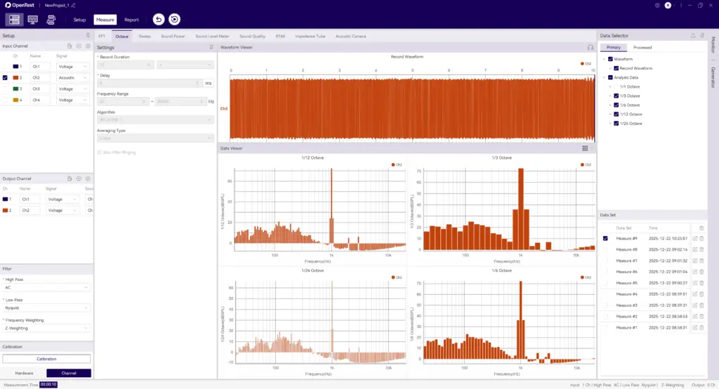
Figure 1: Octave-Band Filter Bank Analysis in OpenTest
FFT binning and FFT synthesis
FFT binning: convert a narrowband spectrum into CPB band integrals
- Estimate spectrum (single FFT, Welch PSD, or STFT).
- Integrate/sum within each octave/fractional-octave band to obtain band power.
This is common in software/offline work because a single FFT provides high-resolution spectrum that can be re-binned into any band system (1/1, 1/3, 1/12, …).
Key challenge #1: FFT scaling and window corrections
After an FFT, scaling depends on your definitions: 1/N normalization, amplitude vs power vs PSD, one-sided vs two-sided spectrum, and windowing. For noise measurements, ENBW is crucial; ignoring it can introduce systematic offsets. [7]
A practical PSD normalization (periodogram form)


# convert to one-sided PSD: multiply by 2 except DC (and Nyquist if present)
This yields PSD in units of (input unit)²/Hz and supports energy consistency checks by integrating PSD over frequency.
Two quick self-checks for scaling
- White noise check: generate noise with known variance σ²; integrate one-sided PSD over 0..fs/2 and recover ≈σ² (accounting for the ×2 rule).
- Pure tone check: generate a sine with amplitude A (RMS=A/√2); integrating spectral energy should recover ≈A²/2 (subject to leakage and window choice).
If both checks pass, your FFT scaling is likely correct; then partial-bin weighting and octave binning become meaningful.
Key challenge #2: band edges rarely align to bins → partial-bin weighting
Hard include/exclude decisions at band edges cause step-like errors, especially at low frequency where bands are narrow. Use overlap-based weighting (Section 4.2.4) for the boundary bins.
Does zero-padding solve edge misalignment? (common misconception)
Zero-padding interpolates the displayed spectrum but does not improve true frequency resolution (which is set by the original window length). It can reduce visual stair-stepping but cannot turn 1–2-bin low-frequency bands into reliable band-level estimates. Fundamental fixes are longer windows or multirate processing/filter banks.
Key challenge #3: time–frequency trade-off (window length sets low-frequency accuracy and delay)
FFT resolution is Δf = fs/N. Low-frequency 1/3-octave bands can be only a few Hz wide, so achieving enough bins per band requires very large N, increasing latency and smoothing transients.
Root cause: 1/3 octave is constant-Q, but STFT uses constant-Δf bins
In CPB, band width scales with frequency (Δf_band ∝ f, constant-Q). In STFT, bin spacing is constant (Δf_bin constant). Therefore low-frequency CPB needs extremely fine Δf_bin (long windows), while high frequency is over-resolved.
Solution routes: long-window STFT vs multirate STFT vs CQT/wavelets
- Long-window STFT: simplest, but high latency and transient smearing.
- Multirate STFT: downsample low-frequency content and FFT at lower fs, similar in spirit to multirate filter banks.
- Constant-Q transform (CQT) / wavelets: naturally logarithmic resolution, but matching IEC/ANSI masks requires extra calibration/validation. [4]
For compliance measurements, standards-oriented filter banks are preferred; for research/feature extraction, CQT/wavelets can be attractive.
FFT synthesis: constructing per-band filtering in the frequency domain
FFT synthesis pushes the FFT approach closer to a filter bank:
- Define a frequency-domain weight W_b[k] per band (brick-wall or smooth/mask-like).
- Compute Y_b[k] = X[k]·W_b[k] and IFFT to get y_b[n].
- Compute band RMS/averages from y_b[n].
It can easily implement zero-phase (non-causal) filtering. For strict IEC/ANSI matching, W_b and normalization must be carefully designed and validated.
Making FFT synthesis stream-like: OLA, dual windows, and amplitude normalization
To output continuous time signals per band, use overlap-add (OLA): frame, window, FFT, apply W_b, IFFT, synthesis window, and OLA. Choose analysis/synthesis windows to satisfy COLA (constant overlap-add) conditions (e.g., Hann with 50% overlap) to avoid periodic level modulation.
If the goal is to match standard filters, how should W_b be chosen?
W_b[k] depends on what you want to match:
- Match brick-wall integration: W_b is hard 0/1 within [f1,f2].
- Match IEC/ANSI filter behavior: |W_b(f)| approximates the standard mask and effective bandwidth (matches ∫|W_b|²).
- Match energy complementarity for reconstruction: design Σ_b |W_b(f)|² ≈ 1 (Section 7.6).
You typically cannot satisfy all three perfectly at once; define your priority (compliance vs decomposition/reconstruction) up front.
Energy-conserving frequency-domain filter banks: why Σ|W_b|² matters
If you want band energies to sum to total energy (within numerical error), a common design aims for approximate power complementarity:

IEC/ANSI masks do not necessarily enforce strict complementarity, so don’t assume exact additivity in compliance contexts.
Welch/averaging strategies: how to make FFT band levels stable
- Use Welch averaging (segment, window, overlap, average power spectra).
- Average in the power domain (|X|² or PSD), then convert to dB.
- For non-stationary signals, consider STFT to obtain time–band matrices.
- Report window type, overlap, averaging count, and ENBW/CG treatment.
FFT-Binning Analysis in OpenTest
OpenTest supports octave-band analysis based on FFT binning:
1) Connect the device, such asSonoDAQ Pro
2) Select the channels and adjust the parameter settings. For an external microphone, enable IEPE and switch to acoustic signal measurement.
3) In the Octave-Band Analysis section under Measurement Mode, choose the FFT-based algorithm.
4) A single recording can be analyzed simultaneously in 1/1-octave, 1/3-octave, 1/6-octave, 1/12-octave, and 1/24-octave bands.
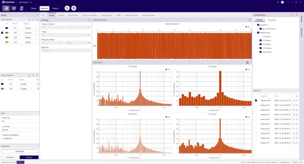
Figure 2: FFT-Binning Octave-Band Analysis in OpenTest
Filter-bank vs FFT/FFT synthesis: differences, equivalence conditions, and trade-offs
A comparison table
| Dimension | Filter-bank (True Octave / CPB) | FFT binning / FFT synthesis |
| Standards compliance | Easier to match IEC/ANSI magnitude masks; mainstream for hardware instruments. [1][3] | Hard binning behaves like band integration; matching masks requires extra weighting or standard-compliant digital filters. |
| Real-time / latency | Causal real-time possible; latency set by filter order and averaging. | Block processing adds at least one window length of delay; low-frequency resolution often forces longer windows. |
| Transient response | Continuous output but affected by group delay/ringing; different compliant implementations may differ. [3] | Set by STFT windowing; transients are smeared by windows and sensitive to window type/length. |
| Leakage & corrections | Controlled via filter design; leakage can be managed. | Strongly depends on window and ENBW/scaling; edge-bin misalignment needs partial weighting. [7] |
| Interpretability | RMS after bandpass filtering—aligned with sound level meters and analyzers. | Spectrum estimation + binning—more statistical; interpretation depends on window/averaging settings. |
| Computation | Many filters in parallel; multirate can reduce cost. | One FFT can serve all bands; efficient for offline/batch. |
| Phase & reconstruction | IIR is typically nonlinear phase (fine for levels). | Frequency weights can be zero-phase; reconstruction needs attention to complementarity and transitions. |
When do both methods give (almost) the same answers?
Band-averaged results typically agree closely when:
- You compare averaged band levels (not transient peak tracks).
- The signal is approximately stationary and the observation time is long enough.
- FFT resolution is fine enough that each band contains enough bins (especially at the lowest band).
- FFT scaling is correct (one-sided handling, Δf, window U, ENBW/CG where needed).
- Partial-bin weighting is used at band edges.
Why differences grow for transients and short events
Differences are driven by mismatched time scales: filter banks have band-dependent group delay and ringing but continuous output; STFT uses a fixed window that sets both frequency resolution and time smoothing. If event duration is comparable to the window length or filter impulse response, results depend strongly on implementation details.
Error budget: where mismatches usually come from (and how to locate them quickly)
- Wrong averaging/combination in dB: must average and sum in the energy domain.
- Inconsistent FFT scaling: 1/N conventions, one-sided vs two-sided, Δf, window normalization U.
- Missing window corrections: ENBW for noise; coherent gain/leakage for tones.
- Using nominal frequencies to compute edges instead of exact definitions.
- No partial-bin weighting at band boundaries (especially harmful at low frequency).
- Multirate/anti-alias issues in filter banks.
- Different averaging time constants/windows between methods.
- True method differences: brick-wall binning vs standard filter skirts/roll-off imply systematic offsets.
A strong debugging approach: first match total mean-square using white noise (scaling/ENBW/partial-bin), then validate band centers and adjacent-band isolation using swept sines or tones.
Engineering checklist: make 1/3-octave analysis correct, stable, and reproducible
Choose a method: compliance → filter bank; offline statistics → FFT binning
- For regulations/type testing/instrument comparability: prefer IEC/ANSI-compliant filter banks and report standard edition and class. [1][3]
- For offline processing, large datasets, or flexible band definitions: FFT binning can be efficient, but scaling and boundary weighting must be rigorous.
- If you need per-band time-domain signals (modulation, envelope, etc.): consider FFT synthesis or explicit filter banks.
Selecting FFT parameters from the lowest band (example)
Example: fs=48 kHz, lowest band of interest is 20 Hz (1/3 octave). Its bandwidth is only a few Hz. If you want at least M=10 bins per band, you may need Δf_bin ≤ bandwidth/10, implying a very large N (e.g., ~100k points; 2^17=131072). This illustrates why real-time compliance often favors filter banks.
Typical mistakes that prevent results from matching
- Summing magnitude |X| instead of power |X|² or PSD.
- Averaging in dB instead of in linear power/mean-square.
- Ignoring ENBW/window scaling for noise. [7]
- Computing band edges from nominal frequencies.
- Not stating time weighting/averaging conventions (Fast/Slow/Leq). [5][6]
Recommended validation flow (regardless of implementation)
- Tone-at-center test (or sweep): verify that energy peaks in the correct band and adjacent-band rejection behaves as expected.
- White/pink noise: verify expected spectral shape in band levels and assess stability/averaging time.
- Cross-implementation comparison: compare your implementation with a known reference on identical signals; isolate scaling vs definition vs filter-skirt differences.
- Record and freeze parameters (band definition, windowing, averaging) in the test report.
Reproducibility checklist: include these in reports so others can recompute your levels
- Band definition: base-10 or base-2? b in 1/b? exact vs nominal used for computation? reference frequency fr?
- Implementation: standard filter bank (IIR/FIR, multirate) vs FFT binning/synthesis; software/library versions.
- Sampling/preprocessing: fs, detrending/DC removal, anti-alias filtering, resampling.
- Time averaging: Leq / block RMS / exponential; time constants, block size, overlap, averaging frames; Fast/Slow context if relevant.
- FFT details (if used): window type, N, hop, zero-padding, PSD normalization, one-sided handling, ENBW/CG, partial-bin weighting.
- Calibration/units: input units and reference quantities (e.g., 20 µPa), sensor calibration factors and dates.
- Output definition: RMS vs peak vs band power; 10log vs 20log conventions; any band aggregation steps.
If you remember one line: document “band definition + time averaging + FFT scaling/window treatment (if any)”. Most disputes disappear.
Quick formulas and numeric example (ready for code/report)
Base-10 one-third-octave constants
G = 10^(3/10) ≈ 1.995262
r = 10^(1/10) ≈ 1.258925 # adjacent center-frequency ratio
k = 10^(1/20) ≈ 1.122018 # edge multiplier about center
f1 = fm / k
f2 = fm * k
Example: the 1 kHz one-third-octave band
fm = 1000 Hz
f1 = 1000 / 1.122018 ≈ 891.25 Hz
f2 = 1000 * 1.122018 ≈ 1122.02 Hz
Δf ≈ 230.77 Hz
Q ≈ 4.33
OpenTest integrates both methods. Download and get started now -> or fill out the form below ↓ to schedule a live demo.
Explore more features and application stories at www.opentest.com.
References
[1] IEC 61260-1:2014 PDF sample (iTeh): https://cdn.standards.iteh.ai/samples/13383/3c4ae3e762b540cc8111744cb8f0ae8e/IEC-61260-1-2014.pdf
[3] ANSI S1.11-2004 preview PDF (ASA/ANSI): https://webstore.ansi.org/preview-pages/ASA/preview_ANSI%2BS1.11-2004.pdf
[4] HEAD acoustics Application Note: FFT - 1/n-Octave Analysis - Wavelet (filter bank description): https://cdn.head-acoustics.com/fileadmin/data/global/Application-Notes/SVP/FFT-nthOctave-Wavelet_e.pdf
[5] IEC 61672-1:2013 (IEC page): https://webstore.iec.ch/en/publication/5708
[6] NTi Audio Know-how: Fast/Slow time weighting (IEC 61672-1 context): https://www.nti-audio.com/en/support/know-how/fast-slow-impulse-time-weighting-what-do-they-mean
[7] MathWorks: ENBW definition example: https://www.mathworks.com/help/signal/ref/enbw.html

OpenTest
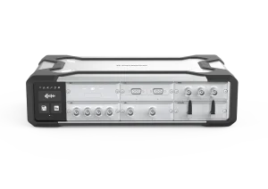
SonoDAQ Pro