Learn how to measure Loudness (ISO 532-1), Sharpness, and Tonality (ECMA-74) with OpenTest — free, open-source software. Step-by-step guide for automotive NVH, consumer electronics & home appliances engineers. This article is for engineers working in acoustics and vibration testing. It introduces how to perform sound quality measurements in OpenTest based on the ISO 532 loudness standard and the ECMA-74 tonality evaluation methods. By measuring and comparing three key psychoacoustic metrics — Loudness, Sharpness, and Prominence (Tonality) — teams in consumer electronics, automotive NVH, home appliances and IT equipment can turn “how good or bad it sounds” into quantitative engineering data, and complete a standardized sound quality workflow on a single platform from data acquisition, through analysis, to reporting.
Why Sound Quality Measurements Matter
In traditional noise testing, we usually rely on dB values to describe how “loud” a device is. But more and more studies and real-world projects are reminding engineers that “loudness” is only part of the story. In automotive NVH, home appliances, IT equipment and consumer electronics, user acceptance of product sound depends much more on whether it sounds pleasant, sharp, tiring or annoying, not just the overall sound pressure level.
Industry surveys also show that most manufacturers now treat “how good it sounds” as being just as important as “how quiet it is”, and they start paying attention to sound quality already in early design phases. At the same sound level, poor sound quality can significantly drag down overall product satisfaction.
This is exactly why Sound Quality as a discipline exists: through a set of psychoacoustic metrics such as Loudness, Sharpness and Tonality/Prominence, it turns subjective impressions like “sharp”, “boomy”, “harsh” or “smooth” into data that is measurable, comparable and traceable, so engineering teams can go beyond noise control and truly design and optimize product sound around listening experience.
Key Metrics in Sound Quality Measurement
In engineering practice, sound quality is not a single number, but a set of psychoacoustic quantities. Commonly used metrics include Loudness, Sharpness, Roughness, Fluctuation Strength, Prominence/Tonality, etc.
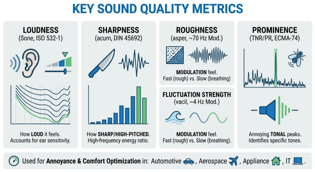
Figure 1 – Key metrics in sound quality measurement
Loudness (ISO 532-1)
Loudness and Loudness Level describe how loud a sound is perceived by the human ear, rather than just its sound pressure level in dB. Internationally, the ISO 532-1:2017 standard based on the Zwicker method is widely used for loudness calculation. It can handle both stationary and time-varying sounds and correlates well with subjective perception in many technical noise applications.
From an engineering point of view, loudness has clear advantages over A-weighted SPL:
- It accounts for the ear’s different sensitivity to frequency (human hearing is more sensitive in the mid-high range)
- At the same dB level, loudness often tracks “does it feel loud or not?” more accurately
Sharpness (DIN 45692)
Sharpness reflects whether a sound is perceived as sharp or piercing. When the high-frequency content has a higher proportion, people tend to feel the sound is more “sharp” or “edgy”.
Sharpness was standardized in DIN 45692:2009, and is typically calculated based on the specific loudness distribution from a loudness model, applying additional weighting in the higher Bark bands. The result is expressed in acum.
In applications such as fans, compressors and e-drive whine, reducing sharpness often improves subjective comfort more effectively than just lowering the overall dB level.
Roughness (asper)
Roughness corresponds roughly to fast amplitude modulation in the 15–300 Hz range, which gives a “raspy, vibrating” impression — for example in certain inverter whines or gear whine where the sound feels like it is “shaking”.
- Unit: asper
- Classical definition: 1 asper corresponds to a 1 kHz, 60 dB pure tone amplitude-modulated at about 70 Hz with 100% modulation depth
- The deeper the modulation and the closer the modulation frequency is to the sensitive region (around 70 Hz), the higher the perceived roughness
In engineering, roughness is often used to describe how much a sound feels like it is “buzzing” or “scratching”, and it is particularly relevant for subjective evaluation of technical noise in e-drive systems, gearboxes and compressors.
Fluctuation Strength (vacil)
Fluctuation Strength captures slower amplitude fluctuations — amplitudes that go up and down in the range of roughly 0.5–20 Hz, perceived as “pulsing” or “breathing”, with a typical peak sensitivity around 4 Hz.
- Unit: vacil
- A classical definition of 1 vacil: a 1 kHz, 60 dB pure tone with 4 Hz, 100% amplitude modulation
- In cabin idle “breathing noise”, or fans whose level periodically rises and falls, fluctuation strength is a key descriptor
You can think of Fluctuation Strength and Roughness as two sides of the same “modulation” coin:
- Fluctuation Strength: slow modulation (a few Hz), perceived as “breathing” or “pulsing”
- Roughness: faster modulation (tens of Hz), perceived as “vibrating, raspy, grainy”
Prominence / Tonality (ECMA-74)
Many devices are not particularly loud overall, yet become extremely annoying because of one or two narrowband tonal components. These “sticking out tones” are usually quantified by Tonality / Prominence.
In IT and information technology equipment noise, ECMA-74 specifies methods based on Tone-to-Noise Ratio (TNR) and Prominence Ratio (PR) to evaluate tonal prominence and to determine whether a spectral line is a “prominent tone”.
Historically, these metrics come from psychoacoustic research and are now widely used in automotive, aerospace, home appliances and IT equipment to predict and optimize annoyance. For example, studies have shown that, with loudness controlled, Sharpness, Tonality and Fluctuation Strength are important predictors for the annoyance of helicopter noise.
Why Sound Quality Is More Useful Than Just “Watching dB”
In many projects, you may have already seen questions like these:
- Two fan designs have similar sound power levels, but one “sounds smooth” while the other has a clear whine
- After noise reduction, overall SPL is a few dB lower, but user feedback hardly improves
- On the production line, A-weighted SPL is used as the only criterion, and some “bad-sounding” units still slip through
Fundamentally, that is because:
- Sound pressure level / sound power = “how much energy is there”
- Sound quality metrics = “how the ear feels about it”
With metrics like Loudness, Sharpness, Roughness, Fluctuation Strength and Prominence, you can decompose vague complaints like “it just sounds uncomfortable” into:
- Which frequency region has too much energy (leading to high sharpness)
- Whether there is strong amplitude modulation (causing high roughness or fluctuation strength)
- Whether any tonal component is sticking out clearly above its surroundings (high tonality / prominence)
In engineering iteration, these metrics can be mapped directly to:
- Structural optimization (stiffness, modes, blade shape, etc.)
- Control strategies (e.g. PWM frequency, fan speed curves and transitions)
- Material and noise treatment / isolation choices
This gives you much clearer and more actionable directions than “just reduce dB”.
Sound Quality Analysis in OpenTest
As a platform for acoustics and vibration testing, OpenTest supports a complete sound quality workflow from acquisition → analysis → reporting. Fill in the form at the bottom ↓ of this page to contact us and get an OpenTest demo.
Example Device: Office PC Fan Noise
To make the process concrete, we use a very accessible device as our example: a typical office PC.
Test objective: evaluate sound quality metrics of its fan noise under different operating conditions, in order to:
- Compare subjective noise performance of different cooling and fan control strategies
- Provide quantitative input to NVH reviews (e.g. does loudness exceed the target, is sharpness too high?)
- Build a foundation for further sound quality optimization (e.g. suppressing whine frequencies, smoothing speed transitions)
Test environments might be:
- A semi-anechoic room / low-noise lab (recommended); or
- A quiet office environment for early-stage, comparative evaluation
Measurement System: SonoDAQ + OpenTest Sound Quality Module
On the hardware side, we use a CRYSOUND SonoDAQ multi-channel data acquisition system (for more detailed model information, please contact us), together with one or more measurement microphones placed near the PC fan or at the listening position, according to the test requirements.
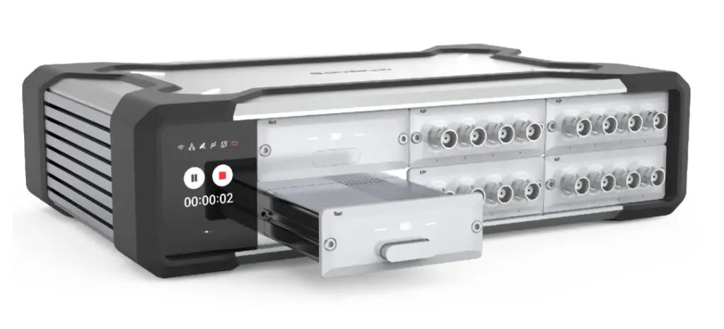
Figure 2 – SonoDAQ Pro multi-channel data acquisition system
Of course, OpenTest also supports connection via openDAQ, ASIO, WASAPI and other mainstream audio interfaces, so you can reuse existing DAQ devices or audio interfaces for measurement where appropriate.
On the software side, the Sound Quality module in OpenTest is one of the measurement modules. Combined with FFT analysis, octave analysis and sound level analysis, it can cover most standard audio and vibration test needs.
Configuring Measurement Parameters
After creating a new project in OpenTest, proceed as follows:
1. Channel configuration and calibration
- In Channel Setup, select the microphone channels to be used and set sensitivity, sampling rate and frequency weighting as required
- Use a sound calibrator (e.g. 1 kHz, 94 dB SPL) to calibrate the measurement microphones, ensuring that loudness and related metrics have a reliable absolute reference
2. Switch to the “Measure > Sound Quality” module
- Select the metrics to be calculated: Loudness, Sharpness, Prominence
- Set analysis bandwidth, frequency resolution and time averaging modes
- Optionally configure test duration and labels for different operating conditions
Essentially, this step turns the “calculation definitions” in ISO 532, DIN 45692 and ECMA-74 into a reusable OpenTest sound quality scenario template.
Acquiring Sound Data for Different Operating Conditions
Once the test environment is set up and the parameters are configured, click Start to measure sound quality data under different operating conditions. Each test record is saved automatically for later analysis.
Because sound quality focuses on how it sounds during real use, it is recommended to record several typical conditions, for example:
- Idle / standby (fan off or low speed)
- Typical office load (documents, multi-tab browsing, etc.)
- High load / stress test (CPU/GPU at full load)
With this breakdown, engineers can clearly manage which sound quality result corresponds to which operating condition.
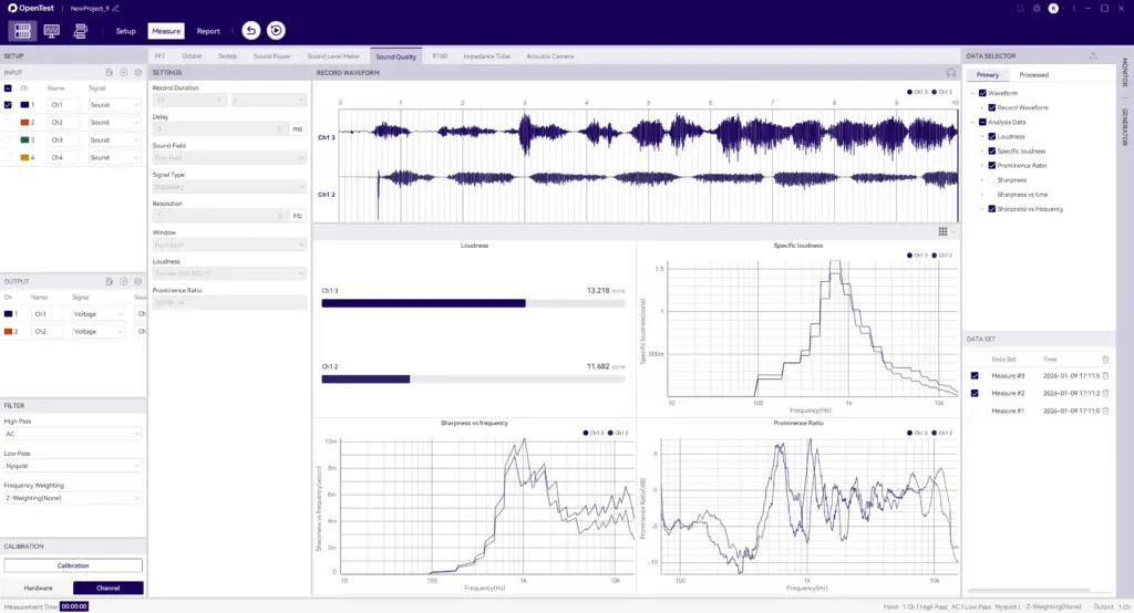
Figure 3 – Overlaying multiple sound quality test records in OpenTest
From Multiple Measurements to One Sound Quality Report
After measuring multiple operating conditions (e.g. idle, typical office and full-load stress test), you can do the following in OpenTest.
- In the data set list, select the records you want to compare and overlay:
- Compare loudness curves under different conditions
- See whether sharpness spikes during acceleration or speed transitions
- Identify conditions where prominent narrowband tones appear (high prominence)
- In the Data Selector, save the associated waveforms and analysis results:
- Export .wav files for later listening tests or subjective evaluations
- Export .csv / Excel for further statistics or modelling
- Click the Report button in the toolbar:
- Enter project, DUT and operating condition information
- Select sound quality metrics and plots to include (e.g. loudness vs. time, bar charts of sharpness, spectra with marked tonal prominence)
- Generate a sound quality report with one click for internal review or customer submission
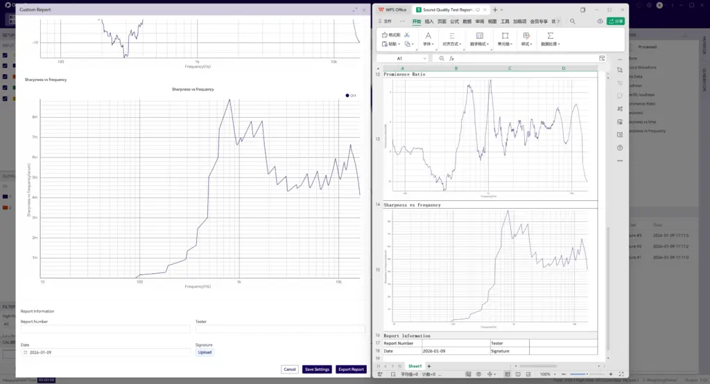
Figure 4 – Example of a sound quality report in OpenTest
The generated report includes measurement conditions and operating modes, key sound quality metrics such as Loudness, Sharpness and Prominence, as well as a comparison with traditional acoustic metrics (sound pressure level, 1/3-octave spectra, sound power, etc.), making it easier for project teams to discuss using a set of metrics that are both objective and closely related to perceived sound.
Typical Application Scenarios
You can build different sound quality test scenarios in OpenTest for different businesses, for example:
- Consumer electronics / IT equipment (laptops, routers, fans, etc.)
- Use loudness + sharpness + (where applicable) roughness to evaluate the “subjective comfort” of different thermal / fan strategies
- Compare sound quality across different speed curves or PWM schemes
- Automotive NVH / e-drive systems
- Use multi-channel acquisition to record interior noise and speed signals synchronously
- Combine order analysis with sound quality metrics to see how “sharp” an e-drive whine is and whether there is pronounced modulation causing roughness
- Home appliances and industrial equipment
- When sound power already meets standards, use sound quality metrics to further screen for “annoying noise”, instead of relying only on dB
If you are building or upgrading your sound quality testing capabilities, you can use ISO 532 and ECMA-74 as the backbone and let OpenTest connect environment, acquisition, analysis and reporting into a repeatable chain. That way, each sound quality test is clearly traceable and much more likely to evolve from a single experiment into a long-term engineering asset.
Welcome to fill in the form below ↓ to contact us and book a demo and trial of the OpenTest Sound Quality module. You can also visit the OpenTest website at www.opentest.com to learn more about its features and application cases.
Get Expert Advice for Your Application
Tell us about your testing requirements and our engineers will recommend the right solution.
OpenTest
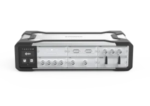
SonoDAQ Pro
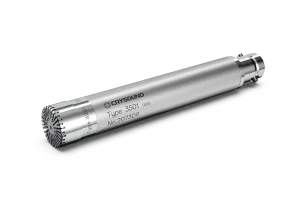
CRY3201-S01 Free-Field Microphone Set, 1/2", 12.5mV/Pa