CRYSOUND POCKET Acoustic Imaging Camera Now Available on Kickstarter.
CRYSOUND POCKET Acoustic Imaging Camera Now Available on Kickstarter.

Sound is everywhere in our daily life: birdsong, street noise, engine roar, even the faint airflow from an air conditioner. For people, sound is not only about whether we can hear it, but whether it feels comfortable, is disturbing, or poses a risk. The same 70 dB can feel completely different; and when something feels "noisy", the cause may come from the source itself, the propagation direction, or reflections from the environment.
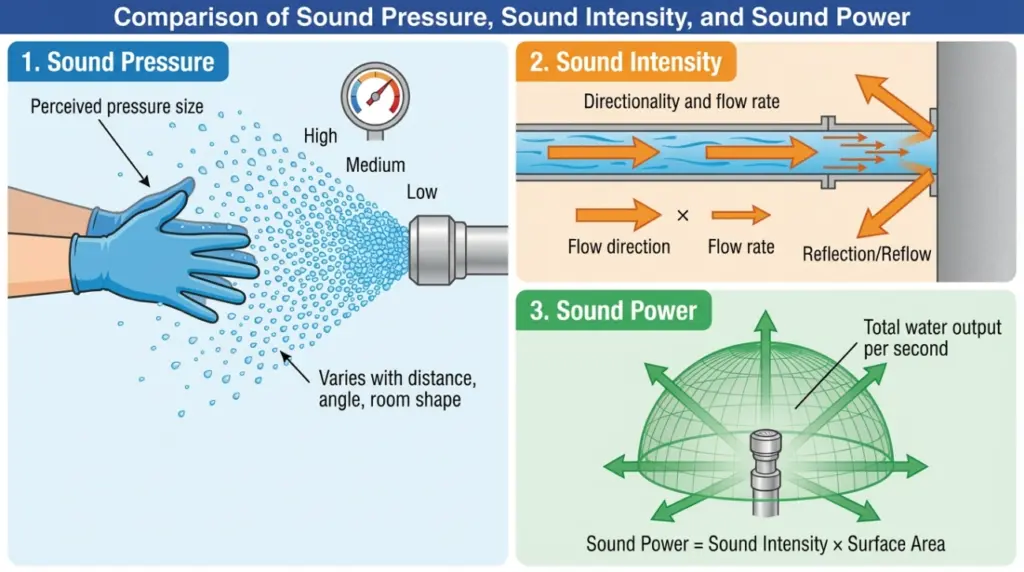
When we turn this "perception" into quantifiable engineering data, the three most easily confused concepts are sound pressure, sound intensity, and sound power. They answer:
- Sound pressure: how loud it is at a specific point;
- Sound intensity: how much sound energy is propagating in a particular direction;
- Sound power: how loud the source is in terms of its total acoustic emission;
This article explains sound pressure, sound intensity, and sound power in an intuitive way, so you can better understand sound.
Sound Waves
In engineering acoustics, sound pressure, sound intensity, and sound power are three fundamental and important physical quantities. Before introducing them in detail, we need the concept of a sound wave.
A vibrating source sets the surrounding air particles into vibration. The particles move away from their equilibrium position, drive adjacent particles, and those adjacent particles generate a restoring force that pushes the particles back toward equilibrium. This near-to-far propagation of particle motion through the medium is what we call a sound wave.
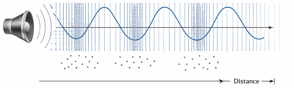
Sound Pressure
When there is no sound wave in space, the atmospheric pressure is the static pressure p0. When a sound wave is present, a pressure fluctuation is superimposed on p0, producing a pressure fluctuation p1. Here p1 is the sound pressure (unit: Pa). Therefore, sound pressure is the instantaneous deviation of the air static pressure caused by the sound wave.
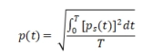
The human brain does not respond to the instantaneous amplitude of sound pressure, but it does respond to the root-mean-square (RMS) value of a time-varying pressure. Therefore, the sound pressure p can be expressed as:
In practical engineering applications, the sound pressure level Lp:
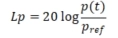
where Pref = 2 × 10⁻⁵ Pa is the reference sound pressure.
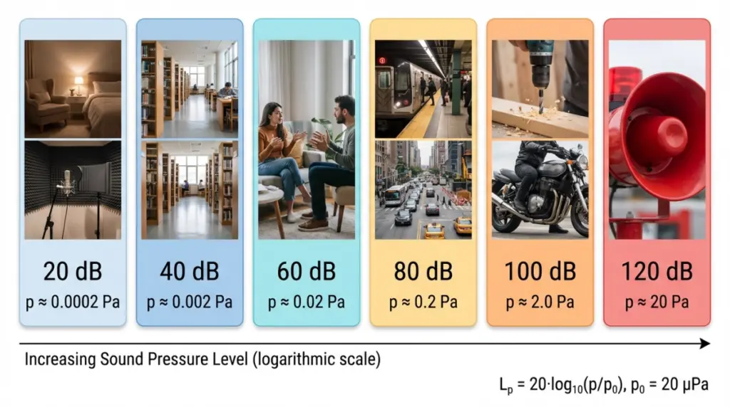
In practice, we usually use sound pressure level (dB) to characterize sound pressure, rather than using pressure in pascals. Why? Figure 2 answers this well. From a library to the entrance of a high-speed rail station, sound pressure may increase by a factor of 100, while sound pressure level increases by only 40 dB. This reflects the difference between a linear scale and a logarithmic scale. From an engineering perspective, using sound pressure directly leads to large numeric variations that are inconvenient for evaluation. Moreover, the human auditory system is closer to a logarithmic response, so sound pressure level better matches hearing.
Sound Intensity
Sound intensity describes the transfer of acoustic energy. It is the acoustic power passing through a unit area per unit time. It is a vector quantity that is directional, with units of W/m2, defined as the time average of the product of sound pressure and particle velocity:
where v(t) denotes the particle velocity vector. Under the ideal plane progressive-wave approximation, sound pressure and particle velocity approximately satisfy:

where ρ is the air density, c is the speed of sound. Therefore, the magnitude of sound intensity along the propagation direction can be written as:

Similarly, sound intensity has a corresponding intensity level LI:

where I0 = 10-12 W/m2 is the reference sound intensity.
Compared with sound pressure level measurements, sound intensity measurements have the following characteristics:
- Directional:it can distinguish whether acoustic energy is propagating outward or flowing back, so under typical field conditions it is often less sensitive to reflections and background noise;
- Source localization:intensity scanning can directly reveal the main radiation regions and leakage points, making remediation more targeted;
- Higher system complexity:it typically requires an intensity probe, with higher overall cost and more setup and calibration effort;
A key advantage of sound intensity measurement in engineering applications is that it characterizes both the direction and magnitude of acoustic energy flow. It can separate the contributions of outward radiation from the source and reflected backflow from the environment, so under non-ideal field conditions it tends to be less affected by reflections and background noise. In addition, the sound intensity method can obtain sound power directly by spatially integrating the normal component of intensity over an enclosing surface. Combined with surface scanning, it can identify dominant source regions and locate leakage points. Therefore, it is highly practical and interpretable for noise diagnosis, verification of noise-control measures, and sound power evaluation.
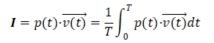
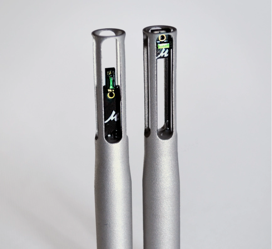
The key instrument for sound intensity testing is the sound intensity probe. Unlike a single microphone, an intensity probe is not used merely to measure "how large the pressure is"; it must provide the basic quantities required for calculating intensity (sound pressure and particle velocity). Therefore, the probe typically outputs two synchronous channels and, together with a two-channel data-acquisition front end and dedicated algorithms, yields intensity results. In engineering practice, the probe often includes interchangeable spacers, positioning fixtures, and windshields. Channel amplitude/phase matching, phase calibration capability, and airflow-interference mitigation directly determine the credibility and usable frequency range of intensity measurements.
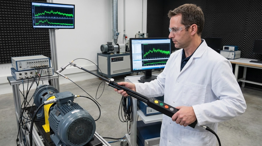
Two types of sound intensity probes are commonly used: P-U probes (pressure-particle-velocity) and P-P probes (pressure-pressure). A P-U probe consists of a microphone and a velocity sensor, measuring sound pressure p(t) and particle velocity v(t) simultaneously. The principle is more direct, but particle-velocity sensors are often more sensitive to airflow, contamination, and environmental conditions, requiring more protection and maintenance in the field and usually costing more.
A P-P probe uses two matched microphones aligned on the same axis. It uses the two pressure signals p1(t) and p2(t) to estimate the particle-velocity component v(t). However, it is sensitive to inter-channel phase matching and the choice of microphone spacing - the spacing determines the effective frequency range: a larger spacing benefits low frequencies, but high frequencies suffer from spatial sampling error; a smaller spacing benefits high frequencies, but low frequencies become more susceptible to phase mismatch and noise.
P-U probes are relatively niche, mainly because it is difficult to make them both stable and inexpensive, and they generally have poorer resistance to airflow. P-P probes, thanks to their good field robustness and the ability to adjust bandwidth flexibly via microphone spacing, are currently the mainstream choice in engineering applications.
Sound Power
Sound power W is the rate at which a source radiates acoustic energy, with units of watts (W). For any closed measurement surface S enclosing the source, the sound power equals the integral of the normal component of sound intensity over that surface:
where n is the unit normal vector pointing outward from the measurement surface.
Sound power level Lw is defined as:
where W0 = 10-12 W is the reference sound power.
Sound power characterizes a source's inherent acoustic emission capability: the total acoustic energy it radiates per unit time. It has little to do with measurement distance or microphone position, and ideally does not depend on how "loud" it is at a particular point in a room. This is fundamentally different from sound pressure and sound intensity.
To better understand sound pressure, sound intensity, and sound power, you can imagine noise as water flow. Sound pressure is like the "water pressure" you feel when you put your hand at a certain location (it changes with distance to the nozzle, direction, and the shape of the basin).
Sound intensity is like the instantaneous "direction and rate of flow" (it has direction and can even be reflected by walls, creating backflow).
Sound power is like "how much water the nozzle sprays per second" - it is a property of the nozzle itself. In measurement, it is obtained by integrating the outward normal flow over a surface surrounding the device.
In real projects, the algorithms for sound pressure, sound intensity, and sound power are relatively mature. The hardest part is acquiring the signals accurately and obtaining results quickly. In particular, tasks such as multi-channel microphone arrays, sound intensity, and sound power impose three hard requirements on the data-acquisition front end: low noise and wide dynamic range, strict synchronization and phase consistency, and stable on-site connections and power.
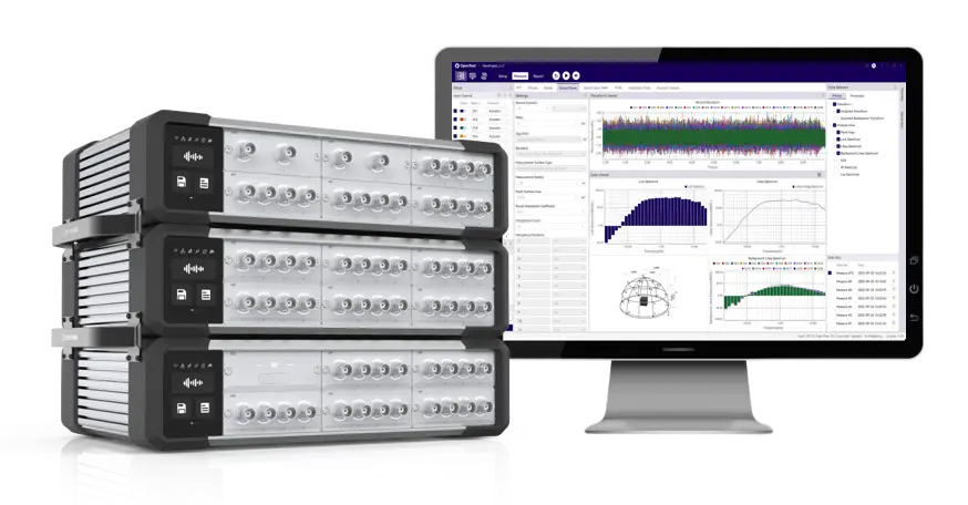
SonoDAQ + OpenTest is positioned to provide a "front-end acquisition + synchronous analysis" foundation for engineering acoustics, allowing engineers to focus more on operating-condition control and data interpretation. It delivers the most value in the following types of projects:
- Sound intensity diagnostics: dual-channel synchronous sampling plus better amplitude/phase consistency management provide a more stable data basis for P-P intensity probes and intensity scanning.
- Microphone array systems: better aligned with engineering deployment needs in channel scalability, synchronization, and cabling, making it suitable for building expandable distributed test platforms.
- Sound power and standardized testing: helps engineers quickly lay out measurement points, covering multiple international sound power test standards. With guided configuration, one-click testing, and automatic report export, it saves substantial time and effort for engineers.
To see more clearly how SonoDAQ is connected and configured, typical application cases (such as equipment noise evaluation, sound source localization, and sound power testing), and commonly used BOM lists, please fill in the form below, and we will recommend the best solution to address your needs.
NEW
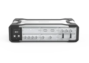
SonoDAQ Pro
lsolation
1000V
Channel
24 channels/Mainframe
Interface
USB-C / 2 x GLAN / 2 x CAN FD / WIFI
NEW

OpenTest
Mode
Measure Mode, Analysis Mode, Sequence Mode
Monitor
Scope, FFT Spectrum, Spectrogram,RMS Level, DC Level, Peak Level, THD Ratio, THD+N Ratio, Crosstalk, etc.
Measure
FFT Analysis, Octave Analysis, Continuous Sweep, Stepped Frequency Sweep, Sound Power Testing, Sound Level Meter, Sound Quality, etc.
NEW
.112_结果_结果_2-scaled-2-300x208.webp)
CRY3213 NVH Measurement Microphone
Field Type
Free-field
Sensitivity
50 mV/Pa, -26±2 dB re 1V/Pa
Frequency Response
3.15 Hz-20 kHz ±2 dB
NEW
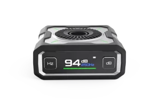
CRY3018 Sound Calibrator
Frequencies
1000 Hz, 250 Hz
Frequency Accuracy
< 0.5 Hz
Sound Pressure Levels (SPL)
94 dB / 114 dB


